DATA → MODEL → ESTIMATE ⇄ EVALUATE → SIMULATE → REPORT
Initial estimates and a first fit
Where you are
The dataset is checked (Preparing and checking the analysis dataset) and the base model is written and validated (Writing and managing model files). This chapter produces the first fit. It covers where starting values come from, how to fit, what the fit object contains, and how to read the warnings ferx attaches to it. Choosing and tuning estimation methods follows in Estimation methods and controlling the fit.
The data
The base model and its dataset from the previous chapters:
base <- ferx_example("two_cpt_oral_base")Starting values
From the model file
Every theta, omega and sigma in [parameters] carries an initial value. For thetas it is the first number in theta NAME(initial, lower, upper):
init_lines <- ferx_model_get_section(base$model, "parameters")
#> # [parameters]
#>   theta TVCL(5.0, 0.1, 100.0)
#>   theta TVV1(50.0, 1.0, 500.0)
#>   theta TVQ(10.0, 0.1, 100.0)
#>   theta TVV2(100.0, 1.0, 500.0)
#>   theta TVKA(1.2, 0.01, 10.0)
#>
#>   omega ETA_CL ~ 0.10
#>   omega ETA_V1 ~ 0.10
#>   omega ETA_Q  ~ 0.05
#>   omega ETA_V2 ~ 0.05
#>   omega ETA_KA ~ 0.15
#>
#>   sigma PROP_ERR ~ 0.02 (sd)
From the data: NCA-based starting values
ferx_inits_from_nca() derives starting values from the data using non-compartmental analysis (NCA). It returns them for inspection without fitting. The method is "nca_sweep" (default), "nca" or "nca_ebe". They differ in how much refinement runs on top of the NCA estimates; ?ferx_inits_from_nca describes each.
nca <- ferx_inits_from_nca(base$model, base$data)
nca
#> <ferx_inits> NCA-based starting values (method = nca_sweep)
#>
#> Theta:
#>       TVCL       TVV1        TVQ       TVV2       TVKA
#>  4.3455257 73.0446185  7.2446104 69.1928716  0.2372377
#>
#> Omega:
#>           ETA_CL ETA_V1 ETA_Q ETA_V2 ETA_KA
#> ETA_CL 0.1029478    0.0  0.00   0.00   0.00
#> ETA_V1 0.0000000    0.1  0.00   0.00   0.00
#> ETA_Q  0.0000000    0.0  0.05   0.00   0.00
#> ETA_V2 0.0000000    0.0  0.00   0.05   0.00
#> ETA_KA 0.0000000    0.0  0.00   0.00   0.15
#>
#> 1 note(s):
#>  - inits_from_nca: 27/30 subjects had a valid AUC estimate; others excluded from NCA pooling
The result is a ferx_inits object, and print() shows the suggested thetas, the omega matrix and any notes. On this dataset all three methods return the same thetas:
To fit from these values directly, pass inits_from_nca to ferx_fit(): TRUE, or one of the method names. The same option exists as the inits_from_nca key in [fit_options] or settings. The Variants section below shows that this is not always an improvement.
A pilot run
ferx_check_init() runs a short pilot fit with the optimizer trace switched on. It returns the fit, the trace (one row per objective evaluation) and a one-row summary:
pilot <- ferx_check_init(base$model, base$data)
#> Warning: Model file [fit_options] sets `covariance = true` but ferx_fit()
#> argument overrides it with `false`. The call-time value will be used.
#> Warning: Model file [fit_options] sets `maxiter = 500` but ferx_fit() argument
#> overrides it with `5`. The call-time value will be used.
pilot$summary
#>   n_iter ofv_start   ofv_end ofv_drop converged
#> 1     98 -1171.882 -1185.403 13.52042      TRUE
The two R warnings come from ferx_check_init() itself. It overrides covariance and maxiter from the model file, and ferx reports every such override. A falling objective function value (OFV) shows that the optimizer moves away from the starting values in a useful direction. On this model the pilot already reached convergence. The trace shows the path:
ggplot(pilot$trace, aes(iter, ofv)) +
  geom_line() +
  coord_cartesian(ylim = range(pilot$trace$ofv[pilot$trace$iter > 10])) +
  labs(x = "Objective evaluation", y = "OFV")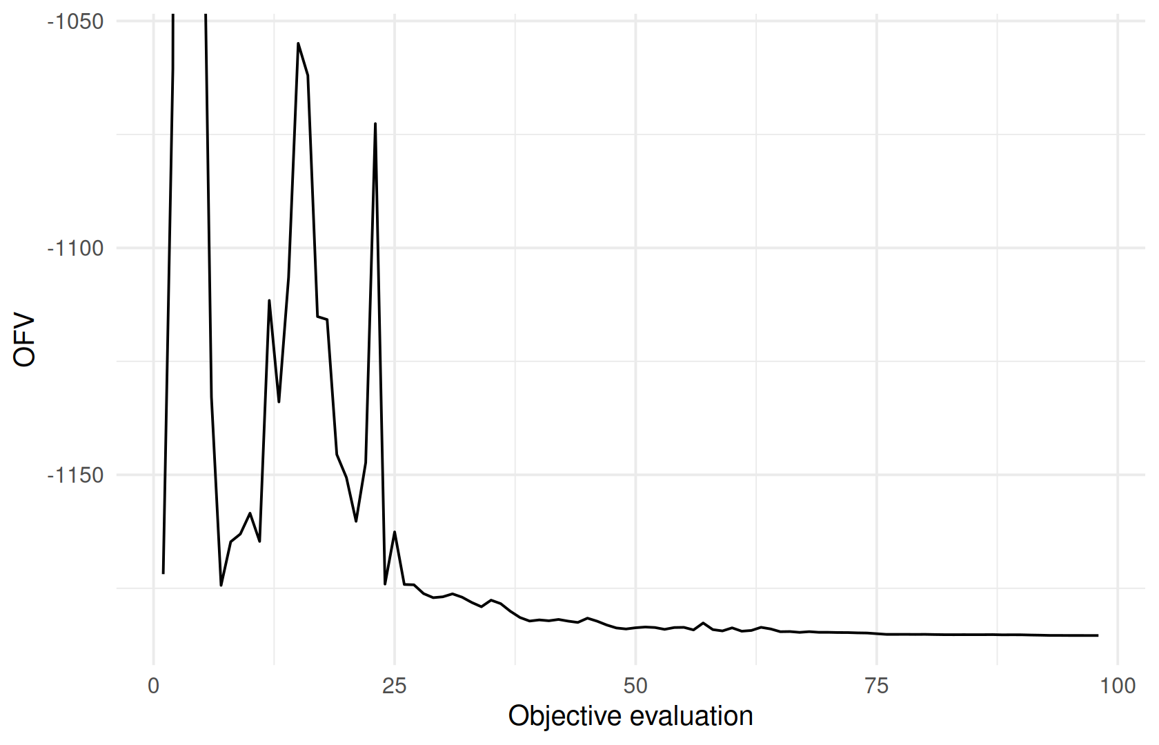
Minimal runnable call
fit <- ferx_fit(base$model, base$data, verbose = FALSE)
fit
#> ============================================================
#>  NONLINEAR MIXED EFFECTS MODEL ESTIMATION
#> ============================================================
#>  Model: two_cpt_oral_base        Dataset: two_cpt_oral_cov
#>  Method: FOCEI | Gradient: FD | Subjects: 30 | Obs: 300
#>
#>  STATUS: CONVERGED   98 iterations   0.8s
#>  OFV: -1185.4028    AIC: -1163.4028    BIC: -1122.6612
#>
#> MODEL STRUCTURE (auto-derived)
#> ------------------------------------------------------------
#>   Structural:  2-cpt oral  (TVCL, TVV1, TVQ, TVV2, TVKA)
#>   IIV:         ETA_CL, ETA_V1, ETA_Q, ETA_V2, ETA_KA
#>   IOV:         none
#>   Residual:    proportional
#>
#> THETA
#> ------------------------------------------------------------
#> Parameter            Estimate           SE       %RSE
#> ----------------------------------------------------
#> TVCL                 4.464758     0.321684        7.2
#> TVV1                48.242245     3.102664        6.4
#> TVQ                  9.584246     0.412960        4.3
#> TVV2                93.787739     3.432550        3.7
#> TVKA                 1.247467     0.097536        7.8
#>
#> OMEGA  (between-subject variability)
#> ------------------------------------------------------------
#>   ETA_CL                   [log-normal]  = 0.155125  CV% = 41.0  SE = 0.040176
#>   ETA_V1                   [log-normal]  = 0.119905  CV% = 35.7  SE = 0.032563
#>   ETA_Q                    [log-normal]  = 0.052574  CV% = 23.2  SE = 0.014448
#>   ETA_V2                   [log-normal]  = 0.038457  CV% = 19.8  SE = 0.010511
#>   ETA_KA                   [log-normal]  = 0.175835  CV% = 43.8  SE = 0.048690
#>
#> SIGMA  (residual error)
#> ------------------------------------------------------------
#>   PROP_ERR         [proportional] = 0.019620  (var = 0.000385, CV% = 2.0)  SE = 0.001123  [initial specified as SD]
#>
#> SHRINKAGE
#> ------------------------------------------------------------
#>  ETA_CL: -0.2%   ETA_V1: 3.6%   ETA_Q: 2.9%   ETA_V2: 2.4%   ETA_KA: 4.2%   EPS: 27.9%
#>
#> DIAGNOSTICS
#> ------------------------------------------------------------
#>  Covariance: computed   Cond: 1.2   DW: 2.91 [negative autocorrelation]   IWRES lag-1 r: -0.532
#>
#> RUN INFO
#> ------------------------------------------------------------
#>  Gradient (requested): fd   (used: fd)
#>  ferx v0.3.0 (core v0.4.0)
#>
#> SETTINGS  (model file / call-time override)
#> ------------------------------------------------------------
#>   method                       focei  [model only]
#>   maxiter                      500  [model only]
#>   covariance                   true  [model only]
#>   gradient                     fd  [model only]
#>
#> ------------------------------------------------------------
#>  1 warning  --  call ferx_get_warnings(fit) for details
#> ============================================================
print() on the fit gives one screen with everything you need to judge it:
- Header: method, gradient, number of subjects and observations, convergence status and OFV/AIC/BIC.
- Model structure, as ferx derived it from the file.
- THETA, OMEGA and SIGMA estimates with standard errors. Omegas are variances; for log-normal etas the CV% is shown alongside.
- Shrinkage, the diagnostics line (covariance step, condition number, Durbin-Watson statistic of the residuals) and run information.
- Settings: every setting, and whether it came from the model file or the call.
- A warning count.
The fit used method = focei and gradient = fd from the model’s [fit_options], marked [model only].
Reading the result
summary()
summary() returns a ferx_summary object. Its print method shows run metadata and all warnings in one compact block, without the parameter tables:
summary(fit)
#> --------------------------------------------------
#> ferx NLME Fit Summary
#> --------------------------------------------------
#> Model:     two_cpt_oral_base
#> Dataset:   two_cpt_oral_cov
#> Converged: YES
#> Method:    FOCEI
#> Gradient:  fd (requested) -> fd (used)
#> ferx v0.3.0 (core v0.4.0)
#>
#> Settings (model file / call-time override):
#>   method                       focei  [model only]
#>   maxiter                      500  [model only]
#>   covariance                   true  [model only]
#>   gradient                     fd  [model only]
#>
#> Structure: 2-cpt oral  (TVCL, TVV1, TVQ, TVV2, TVKA)  |  IIV: ETA_CL, ETA_V1, ETA_Q, ETA_V2, ETA_KA  |  IOV: none  |  Residual: proportional
#>
#> OFV: -1185.4028  AIC: -1163.4028  BIC: -1122.6612
#> Subjects: 30  Obs: 300  Params: 11  Iter: 98
#> Shrinkage: ETA1=-0.2%  ETA2=3.6%  ETA3=2.9%  ETA4=2.4%  ETA5=4.2%
#> EPS shrinkage: 27.9%
#> DW: 2.91 [negative autocorrelation]
#> lag-1 r: -0.532
#> Covariance: computed  Cond: 1.2  |  Wall time: 0.8s
#>
#> Warnings:
#>   * Negative IWRES autocorrelation detected (Durbin-Watson = 2.91). Possible over-parameterization or misspecified error model.
#>   * 19 EBE fallback(s)
#> --------------------------------------------------
The last warning line, the number of EBE fallbacks, comes from fit$total_ebe_fallbacks (19 here). It is a run statistic rather than a structured fit warning, so ferx_get_warnings() below does not list it.
Parameter estimates
fit$estimates is the tidy table of all estimated parameters. The row names are the parameter names:
fit$estimates[, c("transform", "estimate", "se", "rse_pct", "lower_95", "upper_95")]
#>             transform    estimate          se   rse_pct    lower_95
#> TVCL         identity  4.46475758 0.321684435  7.204970  3.83425609
#> TVV1         identity 48.24224473 3.102664029  6.431425 42.16102324
#> TVQ          identity  9.58424559 0.412959827  4.308736  8.77484433
#> TVV2         identity 93.78773933 3.432550369  3.659914 87.05994061
#> TVKA         identity  1.24746711 0.097536293  7.818747  1.05629598
#> ETA_CL       variance  0.15512485 0.040176467 25.899440  0.07637897
#> ETA_V1       variance  0.11990529 0.032563473 27.157662  0.05608088
#> ETA_Q        variance  0.05257442 0.014448475 27.481947  0.02425541
#> ETA_V2       variance  0.03845706 0.010511095 27.332027  0.01785532
#> ETA_KA       variance  0.17583463 0.048690437 27.691040  0.08040137
#> PROP_ERR proportional  0.01961999 0.001122791  5.722687  0.01741932
#>              upper_95
#> TVCL       5.09525907
#> TVV1      54.32346623
#> TVQ       10.39364686
#> TVV2     100.51553806
#> TVKA       1.43863825
#> ETA_CL     0.23387072
#> ETA_V1     0.18372970
#> ETA_Q      0.08089343
#> ETA_V2     0.05905881
#> ETA_KA     0.27126789
#> PROP_ERR   0.02182066
ferx_coef() and ferx_se() pull values by param name. Unlike indexing the table, a misspelt name is an error that suggests the closest match:
Parameter transformations and the transform column
A parameter is not always reported on the scale you want to read. The transform column of fit$estimates names the parameterisation the row came from, which is what you need in order to know whether estimate is the number you want:
transform |
estimate holds |
Which parameters |
|---|---|---|
identity |
the value itself | a theta written as TVCL * exp(ETA_CL)
|
log |
the log of the value | a theta written as exp(TVCL + ETA_CL)
|
logit |
the logit of the value | a theta written as inv_logit(THETA_F + ETA_F)
|
logit_probability |
the value itself, on (0, 1) | a theta declared on the (0, 1) scale and used as inv_logit(logit(THETA_F) + ETA_F)
|
variance |
a variance |
omega and kappa diagonals |
proportional |
a coefficient of variation on the fraction scale | a proportional sigma
|
additive |
a standard deviation, in the units the error model sees | an additive sigma
|
The first four are the transforms a fixed effect can carry, and fit$theta_transforms lists them for the thetas alone. Bounds do not appear here: this column reflects how the parameter is written in [individual_parameters], not the internal scale the optimizer packs it onto, and every bounded theta of this model reads identity:
fit$theta_transforms
#>       TVCL       TVV1        TVQ       TVV2       TVKA
#> "identity" "identity" "identity" "identity" "identity"
log and logit put estimate on the transformed scale and the interpretable value in estimate_natural, with lower_95_natural and upper_95_natural beside it. Those columns are NA for identity, variance, proportional and additive rows, which need no back-transform. logit_probability needs none either – the theta is declared on (0, 1) and the engine returns it there, so estimate is already the number you want and estimate_natural repeats it. The bioavailability example (Absorption and bioavailability) uses that form:
fit_logit <- ferx_fit(ferx_example("bioavailability")$model,
                      ferx_example("bioavailability")$data, verbose = FALSE)
fit_logit$estimates[, c("transform", "estimate", "lower_95", "estimate_natural", "lower_95_natural")]
#>                  transform    estimate    lower_95 estimate_natural
#> TVCL              identity  5.71314425  2.27065256               NA
#> TVV               identity 56.67240359 23.09324119               NA
#> TVKA              identity  1.50009213  1.35597045               NA
#> THETA_F  logit_probability  0.79235918  0.30527844        0.7923592
#> ETA_CL            variance  0.06811478  0.02320218               NA
#> ETA_F             variance  0.15663331 -0.53251792               NA
#> PROP_ERR      proportional  0.12736042  0.10978296               NA
#>          lower_95_natural
#> TVCL                   NA
#> TVV                    NA
#> TVKA                   NA
#> THETA_F         0.1650254
#> ETA_CL                 NA
#> ETA_F                  NA
#> PROP_ERR               NA
THETA_F is the typical bioavailability, 0.792. The model file declares it on that scale (theta THETA_F(0.70, 0.001, 0.999)), and the engine’s own individual parameters agree: reconstructing each subject’s F from estimate reproduces them exactly.
For a log theta the back-transform is real, and estimate_natural is exactly exp(estimate):
log_model <- file.path(book_tempdir("first-fit"), "log_theta.ferx")
writeLines(sub("  CL = TVCL * exp(ETA_CL)", "  CL = exp(TVCL + ETA_CL)",
               sub("  theta TVCL(0.134, 0.001, 10.0)", "  theta TVCL(-2.0, -7.0, 2.3)",
                   readLines(ferx_example("warfarin")$model), fixed = TRUE),
               fixed = TRUE), log_model)
fit_log <- ferx_fit(log_model, ferx_example("warfarin")$data, verbose = FALSE)
log_row <- fit_log$estimates["TVCL", ]
c(transform = log_row$transform,
  difference = log_row$estimate_natural - exp(log_row$estimate))
#>  transform difference
#>      "log"        "0"
The two confidence intervals on a row are built differently. lower_95 and upper_95 are always the symmetric interval estimate ± 1.96 × se on the scale estimate is reported on. On a bounded parameter that interval is not held inside the bounds, so for a probability read it as a measure of precision rather than as limits. For a logit_probability theta, lower_95_natural and upper_95_natural are formed on the logit scale instead – the standard error is carried there by the delta method, se / (p (1 - p)), and the interval brought back with inv_logit() – so they cannot leave [0, 1], and reach its edge only for an estimate close to a bound with a large standard error:
fit_logit$estimates["THETA_F", c("estimate", "lower_95", "upper_95",
                                 "lower_95_natural", "upper_95_natural")]
#>          estimate  lower_95 upper_95 lower_95_natural upper_95_natural
#> THETA_F 0.7923592 0.3052784  1.27944        0.1650254        0.9866093
Here upper_95 is 1.279, a bioavailability above 1, while the natural-scale interval runs from 0.165 to 0.987; for a probability, quote that one. print() shows it on a (95% CI) line under the theta.
That interval is wide for a reason unrelated to how it is built: with oral data only, F, CL and V cannot be separated (Absorption and bioavailability), and the fit says so:
ferx_get_warnings(fit_logit, as_df = TRUE)[, c("category", "severity")]
#>           category severity
#> 1 high_correlation  warning
#> 2 condition_number critical
Declaring the same bioavailability on a logit theta instead, in a separate fit, gives nearly the same natural-scale columns. The agreement is approximate – the delta method is a first-order approximation, and two fits stop at slightly different optima – and only the natural-scale columns are comparable: estimate, lower_95 and upper_95 are on different scales in the two rows.
logit_model <- file.path(book_tempdir("first-fit"), "bioavailability_logit.ferx")
bio_lines <- readLines(ferx_example("bioavailability")$model)
twin_lines <- sub("theta THETA_F(0.70, 0.001, 0.999)  # typical bioavailability, directly on (0,1) scale",
                  "theta THETA_F(0.847, -5.0, 5.0)  # typical bioavailability on the logit scale",
                  bio_lines, fixed = TRUE)
twin_lines <- sub("inv_logit(logit(THETA_F) + ETA_F)", "inv_logit(THETA_F + ETA_F)",
                  twin_lines, fixed = TRUE)
stopifnot(sum(twin_lines != bio_lines) == 2)   # both lines really were rewritten
writeLines(twin_lines, logit_model)
fit_twin <- ferx_fit(logit_model, ferx_example("bioavailability")$data, verbose = FALSE)
natural <- c("transform", "estimate_natural", "lower_95_natural", "upper_95_natural")
natural_gap <- max(abs(unlist(fit_logit$estimates["THETA_F", natural[-1]]) -
                       unlist(fit_twin$estimates["THETA_F", natural[-1]])))
rbind(declared_on_0_1 = fit_logit$estimates["THETA_F", natural],
      declared_as_logit = fit_twin$estimates["THETA_F", natural])
#>                           transform estimate_natural lower_95_natural
#> declared_on_0_1   logit_probability        0.7923592        0.1650254
#> declared_as_logit             logit        0.7923566        0.1654716
#>                   upper_95_natural
#> declared_on_0_1          0.9866093
#> declared_as_logit        0.9865661
The largest difference between the two rows’ natural-scale columns is 0.00045.
For the random effects, fit$eta_param_types says how each eta enters the model – log_normal, additive, logit, logit_probability or custom:
fit$eta_log_transformed is a narrower flag and not a substitute: it is TRUE only for the TVCL * exp(ETA_CL) form, so an eta written exp(TVCL + ETA_CL) is log-normal and still reads FALSE.
Nothing here converts for you. An omega row is a variance, so a between-subject CV% is yours to compute (Tables and figures), and a log-transform-both-sides model reports an additive sigma on the log scale rather than in the units of DV (Variability: random effects, residual error and IOV).
The fit object
A fit is a named list with 112 elements. These are the ones you will use most:
| What you want | Where |
|---|---|
| Parameter table | fit$estimates |
Residuals, PRED, IPRED per observation |
fit$sdtab (Diagnosing the model) |
| Individual parameters per subject | fit$individual_estimates |
| Random effects per subject | fit$ebe_etas |
| OFV, AIC, BIC, convergence |
fit$ofv, fit$aic, fit$bic, fit$converged
|
| Shrinkage |
fit$shrinkage_eta, fit$shrinkage_eps
|
| Parameter correlations | fit$cor_matrix |
head(fit$individual_estimates)
#>   ID       CL       V1         Q        V2        KA
#> 1  1 4.361100 42.73915 11.328502  88.82908 2.2309504
#> 2  2 5.971974 60.77905 12.027252  85.12710 3.3378917
#> 3  3 4.943563 50.09243  8.064386  68.61452 1.2038166
#> 4  4 3.057613 21.53132  7.877632  86.96907 0.9459055
#> 5  5 5.822952 39.95172 11.235375  65.71344 1.2051688
#> 6  6 7.726836 45.63701  8.423314 113.38803 1.4900726
?ferx_fit documents every element. Function, option and example index lists them all with the chapter that uses each one.
Warnings
ferx classifies everything it notices during a fit. Each warning has a severity and a stable category token:
| Severity | Meaning |
|---|---|
| critical | The result cannot be trusted as it is (for example no convergence or an ill-conditioned covariance) |
| warning | The result stands, but a caveat applies |
| info | A note; no action needed |
ferx_get_warnings() prints them grouped by severity. With as_df = TRUE it returns a data frame you can filter:
ferx_get_warnings(fit)
#> ferx fit warnings  (two_cpt_oral_base)
#> -------------------------------------------------
#> [WARNING]  dw_autocorrelation
#>             Negative IWRES autocorrelation detected (Durbin-Watson = 2.91).
#>             Possible over-parameterization or misspecified error model.
#>             Negative IWRES autocorrelation suggests over-parameterisation or a
#>             misspecified error model. Consider removing a parameter or
#>             simplifying the residual model.
#>
#> -------------------------------------------------
#> 0 CRITICAL   1 WARNING   0 INFO
ferx_get_warnings(fit, as_df = TRUE)[, c("severity", "category")]
#>   severity           category
#> 1  warning dw_autocorrelation
fit$warnings holds the same messages as plain text. Because the category tokens are stable, scripts can branch on them. For example, reject any fit with a critical warning. check_diagnostics() returns the residual autocorrelation and shrinkage behind two common warnings as data frames:
check_diagnostics(fit)
#> $autocorrelation
#>   dw_statistic     lag1_r                     flag
#> 1     2.909623 -0.5317191 negative autocorrelation
#>
#> $shrinkage
#>      param type    shrinkage shrinkage_pct
#> 1   ETA_CL  eta -0.001744168    -0.1744168
#> 2   ETA_V1  eta  0.036475626     3.6475626
#> 3    ETA_Q  eta  0.029265476     2.9265476
#> 4   ETA_V2  eta  0.024072075     2.4072075
#> 5   ETA_KA  eta  0.041527717     4.1527717
#> 6 PROP_ERR  eps  0.278869975    27.8869975
What these diagnostics mean and how to act on them is the subject of Diagnosing the model.
Options that matter
Arguments of ferx_fit() introduced here. A call-time value always overrides the model file’s [fit_options], and ferx reports the override:
| Argument | Default | Meaning |
|---|---|---|
model |
— | Model file or ferx_model object |
data |
NULL |
Dataset; NULL uses the ferx_model object’s data or the model’s [data] block |
method |
NULL |
Estimation method(s); NULL uses the model file, otherwise "focei" (Estimation methods and controlling the fit) |
covariance |
NULL |
Run the covariance step (standard errors); NULL uses the model file, which defaults to TRUE
|
verbose |
NULL |
Print progress; NULL uses the model file, which defaults to TRUE
|
inits_from_nca |
FALSE |
Replace starting values with NCA-based ones (TRUE or a method name) |
The other ferx_fit() arguments are covered where they matter: threads, gradient, optimizer_trace and settings in Estimation methods and controlling the fit; ignore, accept and ignore_ids in Preparing and checking the analysis dataset; bloq_method in Censored observations (BLOQ); mu_referencing and scale_params in Variability: random effects, residual error and IOV; sir and fd_hessian_step in Parameter uncertainty; output and include_data in Reproducibility and sharing.
For example, skipping the covariance step:
fit_nocov <- ferx_fit(base$model, base$data, covariance = FALSE, verbose = FALSE)
#> Warning: Model file [fit_options] sets `covariance = true` but ferx_fit()
#> argument overrides it with `false`. The call-time value will be used.
fit_nocov$covariance_status
#> [1] "not_requested"
head(fit_nocov$estimates[, c("estimate", "se")], 3)
#>       estimate se
#> TVCL  4.464758 NA
#> TVV1 48.242245 NA
#> TVQ 9.584246 NA| Function | Arguments |
|---|---|
ferx_inits_from_nca() |
model, data, method ("nca_sweep", "nca", "nca_ebe") |
ferx_check_init() |
model, data, method (default "focei"), maxiter (pilot iteration limit), further arguments passed to ferx_fit()
|
ferx_coef(), ferx_se()
|
fit, param (names; NULL for all) |
ferx_get_warnings() |
fit, as_df
|
check_diagnostics() |
fit |
Variants
Starting from NCA-based values
Fit the base model three ways: from the model file’s starting values, from NCA-based starting values, and from NCA-based values with gradient = "auto" instead of the model file’s finite differences:
fit_nca <- ferx_fit(base$model, base$data, inits_from_nca = TRUE, verbose = FALSE)
fit_nca_auto <- ferx_fit(base$model, base$data, inits_from_nca = TRUE, gradient = "auto",
                         verbose = FALSE)
#> Warning: Model file [fit_options] sets `gradient = fd` but ferx_fit() argument
#> overrides it with `auto`. The call-time value will be used.

worst <- function(f) {
  sev <- ferx_get_warnings(f, as_df = TRUE)$severity
  if ("critical" %in% sev) "critical" else if ("warning" %in% sev) "warning" else "none"
}
data.frame(
  start = c("model file", "NCA", "NCA, gradient = auto"),
  converged = c(fit$converged, fit_nca$converged, fit_nca_auto$converged),
  ofv = c(fit$ofv, fit_nca$ofv, fit_nca_auto$ofv),
  worst_warning = c(worst(fit), worst(fit_nca), worst(fit_nca_auto))
)
#>                  start converged       ofv worst_warning
#> 1           model file      TRUE -1185.403       warning
#> 2                  NCA      TRUE -1080.741      critical
#> 3 NCA, gradient = auto      TRUE -1185.462       warning
All three report converged = TRUE (with gradient = "auto", ferx used the analytic gradient). The NCA start with finite differences, however, ended at an OFV about 105 points higher than the other two, with a critical warning. Its warnings show why the result cannot be trusted:
nca_warnings <- ferx_get_warnings(fit_nca, as_df = TRUE)
nca_warnings[, c("severity", "category")]
#>   severity               category
#> 1  warning                general
#> 2  warning    ebe_start_dependent
#> 3  warning covariance_regularized
#> 4  warning           inflated_rse
#> 5  warning     dw_autocorrelation
#> 6  warning       high_correlation
#> 7 critical       condition_number
#> 8  warning          eta_normality
# The paragraph below names this category, so its absence has to fail the render.
stopifnot("ebe_start_dependent" %in% nca_warnings$category)
The NCA-based absorption rate constant (TVKA = 0.237) is far from the estimate of the successful fits (1.247). Convergence only means the optimizer stopped. Always compare the OFV and read the warnings before accepting a fit.
ebe_start_dependent in that list is a second reason to distrust this one: the random effects it reports depend on where the inner loop started, so every per-subject diagnostic built on them (Diagnosing the model) inherits that dependence. Estimation methods and controlling the fit shows what to change.
Pitfalls
A fit stopped by its iteration limit. maxiter caps the outer optimizer. The engine turns it into a budget of objective evaluations, whose size depends on the optimizer, which is why the warning below speaks of an evaluation budget. A fit that hits the limit is marked unconverged with a critical convergence warning. For the warfarin example with method = "focei":
warf <- ferx_example("warfarin")
fit_short <- ferx_fit(warf$model, warf$data, method = "focei",
                      settings = list(maxiter = 2), verbose = FALSE)
#> Warning: Model file [fit_options] sets `method = foce` but ferx_fit() argument
#> overrides it with `focei`. The call-time value will be used.
#> Warning: Model file [fit_options] sets `maxiter = 300` but ferx_fit() argument
#> overrides it with `2`. The call-time value will be used.
# The sentence above says this fit is unconverged, so a converged one has to fail the render.
stopifnot(!fit_short$converged)
fit_short$converged
#> [1] FALSE
ferx_get_warnings(fit_short, as_df = TRUE)[, c("severity", "category", "message")]
#>   severity           category
#> 1  warning            general
#> 2 critical        convergence
#> 3  warning dw_autocorrelation
#>                                                                                                                       message
#> 1           Outer optimization hit the evaluation budget (maxiter = 2) before converging; increase maxiter for a tighter fit.
#> 2                                                                                         Outer optimization did not converge
#> 3 Negative IWRES autocorrelation detected (Durbin-Watson = 2.61). Possible over-parameterization or misspecified error model.
For the same reason fit_short$n_iterations is 16 here, not 2.
Other points:
-
n_iterationsand the rows of the optimizer trace count objective evaluations, not outer iterations, so they can be much larger thanmaxiter. - Reading
fit$estimates["NAME", ]with a misspelt name silently returnsNA.ferx_coef()andferx_se()stop with an error instead.
Warnings you may see here
-
convergence(critical): the optimizer did not converge. Reject the fit, then change starting values, method or bounds and refit. See convergence and covariance warnings. -
general(warning): the fallback category for messages not assigned to a specific code. Examples in this book are notes from NCA starting values, the location of an optimizer trace file, a stopped fit, and a misspelt data-selection column (Preparing and checking the analysis dataset). Read the message. See solver, numerics and unclassified warnings.
Summary
- Starting values come from
[parameters].ferx_inits_from_nca()proposes data-based ones, andferx_check_init()runs a pilot. -
ferx_fit(model, data)fits.print()andsummary()show the result, andfit$estimates,ferx_coef()andferx_se()give the numbers. - Judge a fit by convergence, OFV and warnings.
ferx_get_warnings(as_df = TRUE)makes them scriptable.
Next: Estimation methods and controlling the fit chooses and tunes the estimation method.
TipReference
- R help:
?ferx_fit,?summary.ferx_fit,?ferx_inits_from_nca,?ferx_check_init,?ferx_coef,?ferx_get_warnings,?check_diagnostics - ferx-core: fit options, warnings