Parameter uncertainty

Where you are

Model development and selection selected the covariate model two_cpt_oral_cov. Before reporting its estimates or simulating from it, quantify how precisely they are known. ferx offers four routes:

the covariance step: asymptotic standard errors from the curvature of the objective function;
SIR: sampling importance resampling around that asymptotic distribution;
the bootstrap: refitting the model to resampled datasets;
Bayesian estimation: posterior intervals.

This chapter applies each to the covariate model and compares the intervals.

The data

cov <- ferx_example("two_cpt_oral_cov")
fit <- ferx_fit(cov$model, cov$data, verbose = FALSE)

Minimal runnable call: the covariance step

The covariance step runs by default (covariance = TRUE in this model file). Its results are the se, rse_pct and 95% interval columns of fit$estimates:

fit$covariance_status
#> [1] "computed"
fit$estimates[, c("estimate", "se", "rse_pct", "lower_95", "upper_95")]
#>               estimate          se   rse_pct    lower_95     upper_95
#> TVCL        4.94779587 0.359479681  7.265451  4.24321569   5.65237604
#> TVV1       48.58746510 2.952179029  6.076010 42.80119420  54.37373599
#> TVQ         9.57692867 0.407841896  4.258588  8.77755856  10.37629879
#> TVV2       94.17330801 3.423849490  3.635690 87.46256301 100.88405301
#> TVKA        1.25592751 0.098051230  7.807077  1.06374710   1.44810792
#> THETA_WT    0.65345631 0.236131062 36.135708  0.19063943   1.11627319
#> THETA_CRCL  0.56461277 0.221501060 39.230615  0.13047069   0.99875484
#> ETA_CL      0.10753130 0.028096449 26.128623  0.05246226   0.16260034
#> ETA_V1      0.10634759 0.028678257 26.966531  0.05013821   0.16255698
#> ETA_Q       0.05124930 0.014007561 27.332201  0.02379448   0.07870412
#> ETA_V2      0.03793979 0.010328799 27.224185  0.01769535   0.05818424
#> ETA_KA      0.17543720 0.048574865 27.687893  0.08023046   0.27064393
#> PROP_ERR    0.01961856 0.001123479  5.726613  0.01741654   0.02182058

The full variance-covariance matrix of the estimates is fit$cov_matrix, and its correlation form is fit$cor_matrix (Diagnosing the model).

Choosing the covariance estimator

book_settings_table(c("covariance_method", "covariance_fallback", "analytic_cov_hessian",
                      "cov_inner_tol", "fd_hessian_step"))

Table 10.1

Setting	Values	Default	Description
`covariance_method`	`r`, `s`, `rsr`	`r`	See `?ferx_fit` and the ferx-core fit options page.
`covariance_fallback`	`none`, `sir`	`none`	What to do when the covariance Hessian is non-PD, whether `R` is analytic or finite-difference.
`analytic_cov_hessian`	`true`, `false`	`true`	Use the exact analytic R-matrix for the covariance step when the model is in scope, instead of the finite-difference-of-OFV Hessian.
`cov_inner_tol`	float	`inner_tol` (LTBS: `min(inner_tol, 1e-8)`)	Inner EBE-reconvergence tolerance used only by the covariance step, decoupled from `inner_tol`.
`fd_hessian_step`	float	`1e-2`	Initial relative step size for the finite-difference Hessian used in the covariance step.

fd_hessian_step is also a dedicated ferx_fit() argument. ferx_covariance() runs the covariance step on an existing fit: to add standard errors to a fit made without them, or to try another estimator without re-estimating. It takes the fitted model as fit, re-reads the model and data files, and stops if they changed since the fit:

fit_nocov <- ferx_fit(cov$model, cov$data, covariance = FALSE, verbose = FALSE)
#> Warning: Model file [fit_options] sets `covariance = true` but ferx_fit()
#> argument overrides it with `false`. The call-time value will be used.
se_by_method <- sapply(c(r = "r", s = "s", rsr = "rsr"), function(m) {
  ferx_covariance(fit_nocov, covariance_method = m)$se_theta
})
round(se_by_method, 4)
#>                 r      s    rsr
#> TVCL       0.3595 0.3819 0.4216
#> TVV1       2.9522 4.5246 2.8639
#> TVQ        0.4078 0.6359 0.3967
#> TVV2       3.4238 4.7218 3.3730
#> TVKA       0.0981 0.1320 0.0954
#> THETA_WT   0.2361 0.2322 0.3255
#> THETA_CRCL 0.2215 0.3284 0.2159

"r" (inverse Hessian, the default) reproduces the inline standard errors, "s" is the inverse cross-product and "rsr" the sandwich estimator. ferx_covariance() also takes mu_referencing (match the original fit) and verbose.

SIR

SIR draws parameter vectors from the asymptotic distribution, weights them by how well they fit the data, and resamples according to the weights. The resampled vectors give intervals that need not be symmetric. Run it inline with ferx_fit(sir = TRUE), or afterwards with ferx_sir(), which takes the fitted model as fit:

fit_sir <- ferx_sir(fit, sir_samples = 1000, sir_resamples = 250)
fit_sir$sir_ess
#> [1] 139.1451
fit_sir$sir_ci_theta
#>                 lower      upper
#> TVCL        4.5718176   5.763030
#> TVV1       41.4399336  56.180391
#> TVQ         8.4433396  10.287684
#> TVV2       86.3826286 100.823310
#> TVKA        1.0614647   1.488455
#> THETA_WT    0.2833786   1.166469
#> THETA_CRCL  0.2839566   1.051120

sir_ci_omega and sir_ci_sigma hold the intervals for the variances and residual error. sir_ess is the effective sample size of the resampled set; the closer it is to sir_resamples, the better the proposal matches the data. sir_keep_samples = TRUE keeps the resampled vectors on the fit, which ferx_simulate_with_uncertainty() needs (Simulating scenarios). verbose = TRUE prints progress.

book_settings_table(c("sir_samples", "sir_resamples", "sir_seed", "sir_keep_samples", "sir_df"))

Table 10.2

Setting	Default	Description
`sir_samples`	`1000`	Number of proposal samples (M)
`sir_resamples`	`250`	Number of resampled vectors (m)
`sir_seed`	`12345`	RNG seed for reproducibility
`sir_keep_samples`	`false`	Retain resampled parameter vectors for `simulate_with_uncertainty()`
`sir_df`	`5.0`	Degrees of freedom for the Student-t proposal; higher values approach a normal proposal

The effective sample size depends strongly on the random seed:

sapply(c(seed_1 = 1, seed_2 = 2), function(s) {
  ferx_sir(fit, sir_samples = 1000, sir_resamples = 250, sir_seed = s)$sir_ess
})
#>   seed_1   seed_2 
#> 17.86333 68.17320

Check sir_ess on every run. When it is low, increase sir_samples and confirm that the intervals are stable across seeds before using them.

Bootstrap

ferx_bootstrap() resamples whole subjects with replacement, refits the model to each replicate and summarises the spread of the estimates. It needs the model and data rather than a fit, because every replicate is a new fit. With a directory it writes its tables to disk, so a run can be re-summarised or resumed later:

boot_dir <- book_tempdir("bootstrap")
boot <- ferx_bootstrap(cov$model, cov$data, samples = 100, seed = 1, directory = boot_dir)
boot
#> ferx bootstrap
#>   Model:  /home/runner/work/_temp/Library/ferx/examples/models/two_cpt_oral_cov.ferx
#>   Data:   /home/runner/work/_temp/Library/ferx/examples/data/two_cpt_oral_cov.csv
#>   Samples: 100 completed of 100 requested; 96 included
#>     excluded 1: estimate near boundary
#>     excluded 3: minimization terminated
#>   Wrote:  /tmp/RtmpqyEfTz/bootstrap
#> 
#> 95% confidence intervals (percentile / normal approximation):
#>             parameter original     mean       bias standard_error   median
#>                  TVCL  4.94800  4.94700 -0.0008091      0.2960000  4.97300
#>                  TVV1 48.59000 48.71000  0.1265000      2.8520000 48.75000
#>                   TVQ  9.57700  9.54800 -0.0290400      0.3984000  9.53700
#>                  TVV2 94.17000 94.64000  0.4632000      3.2470000 94.99000
#>                  TVKA  1.25600  1.26400  0.0082320      0.0894700  1.25300
#>              THETA_WT  0.65350  0.69330  0.0398100      0.2338000  0.67900
#>            THETA_CRCL  0.56460  0.55550 -0.0090700      0.2119000  0.54190
#>  OMEGA(ETA_CL,ETA_CL)  0.10750  0.10000 -0.0075130      0.0246800  0.09761
#>  OMEGA(ETA_V1,ETA_V1)  0.10630  0.09839 -0.0079560      0.0298000  0.09374
#>    OMEGA(ETA_Q,ETA_Q)  0.05125  0.04872 -0.0025250      0.0147400  0.04855
#>  OMEGA(ETA_V2,ETA_V2)  0.03794  0.03857  0.0006253      0.0100600  0.03828
#>  OMEGA(ETA_KA,ETA_KA)  0.17540  0.16830 -0.0071040      0.0589800  0.16000
#>              PROP_ERR  0.01962  0.01948 -0.0001430      0.0009443  0.01951
#>  ci_lower  ci_upper ci_lower_normal ci_upper_normal
#>   4.24200   5.55100         4.36800         5.52800
#>  42.40000  54.80000        43.00000        54.18000
#>   8.95400  10.56000         8.79600        10.36000
#>  88.43000 101.40000        87.81000       100.50000
#>   1.12800   1.51000         1.08100         1.43100
#>   0.23850   1.14400         0.19520         1.11200
#>   0.13220   1.00200         0.14940         0.97990
#>   0.06054   0.15790         0.05917         0.15590
#>   0.05669   0.16720         0.04793         0.16480
#>   0.02403   0.08200         0.02236         0.08014
#>   0.01733   0.05806         0.01821         0.05766
#>   0.07201   0.30790         0.05985         0.29100
#>   0.01736   0.02139         0.01777         0.02147

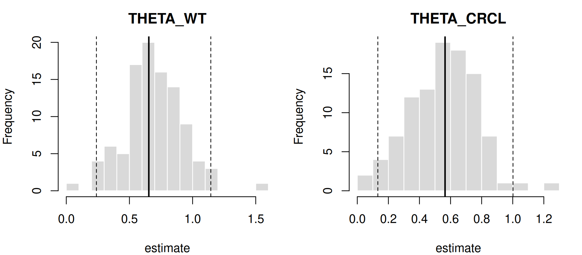
print() on the ferx_bootstrap result shows the run summary and the boot$parameters table: original estimate, bootstrap mean, bias, standard error, median, and the percentile and normal-approximation intervals. boot$raw has one row per fitted replicate, and boot$diagnostics records the counts and exclusions:

boot$diagnostics
#>                            statistic        value
#> 1                  samples_requested   100.000000
#> 2                  samples_completed   100.000000
#> 3                   samples_included    96.000000
#> 4                      chi_square_df    13.000000
#> 5   excluded: estimate near boundary     1.000000
#> 6  excluded: minimization terminated     3.000000
#> 7      mean: minimization_successful     0.970000
#> 8       mean: estimate_near_boundary     0.010000
#> 9   mean: covariance_step_successful     0.000000
#> 10    mean: covariance_step_warnings     0.000000
#> 11                         mean: ofv -1214.723795
#> 12         mean: subproblem_est_time     1.060082

By default, replicates whose minimization terminated or whose estimate lies on a boundary are fitted but excluded from the statistics. plot() on a ferx_bootstrap object draws one histogram per parameter, with the original estimate and the interval:

plot(boot, parameters = c("THETA_WT", "THETA_CRCL"))

Figure 10.1: Bootstrap distributions of the covariate exponents.

ferx_bootstrap_summarize() recomputes the statistics from the run directory under different exclusion criteria or a different ci level, without refitting:

relaxed <- ferx_bootstrap_summarize(boot_dir, skip_estimate_near_boundary = FALSE, ci = 90)
relaxed$n_included
#> [1] 97
head(relaxed$parameters[, c("parameter", "ci_lower", "ci_upper")], 7)
#>    parameter   ci_lower   ci_upper
#> 1       TVCL  4.3922034   5.455515
#> 2       TVV1 43.7777937  53.194542
#> 3        TVQ  8.9953717  10.291399
#> 4       TVV2 89.4531726 100.678700
#> 5       TVKA  1.1386823   1.442725
#> 6   THETA_WT  0.2963447   1.069042
#> 7 THETA_CRCL  0.1761630   0.892184

ferx_bootstrap() arguments:

Argument	Default	Meaning
`model`, `data`	—	Model and dataset (`data = NULL` uses `[data]`)
`samples`	200	Number of bootstrap datasets
`seed`	1	Master seed; results do not depend on `threads`
`threads`	`NULL`	Replicates fitted concurrently
`stratify_on`	`NULL`	Column defining resampling strata
`sample_size`	`NULL`	Subjects per replicate (a named vector gives counts per stratum)
`update_inits`	`TRUE`	Start each replicate from the original fit’s estimates
`run_base_model`	`TRUE`	Fit the original dataset first (needed for bias and `update_inits`)
`keep_covariance`	`FALSE`	Run the covariance step per replicate
`dofv`	`FALSE`	Evaluate each replicate’s estimates on the original data (about doubles the run time)
`skip_minimization_terminated`	`TRUE`	Exclude replicates whose minimization terminated
`skip_estimate_near_boundary`	`TRUE`	Exclude replicates with an estimate on a boundary
`skip_covariance_step_terminated`, `skip_with_covstep_warnings`	`FALSE`	Exclude on the per-replicate covariance step (needs `keep_covariance = TRUE`)
`ci`	95	Confidence level in percent
`directory`	`NULL`	Where to write the run; `NULL` keeps it in memory
`resume`, `retry_failed`	`FALSE`	Continue an interrupted run in `directory`, optionally refitting failed replicates
`progress`, `verbose`	—	Progress bar (interactive sessions) and a run header

ferx_bootstrap_summarize() takes the run directory plus the four skip_* filters and ci.

Bayesian estimation

method = "bayes" returns posterior summaries instead of a covariance step (Estimation methods and controlling the fit). Posterior intervals are only meaningful when the chains have converged:

fit_bayes <- ferx_fit(cov$model, cov$data, method = "bayes", verbose = FALSE)
#> Warning: Model file [fit_options] sets `method = focei` but ferx_fit() argument
#> overrides it with `bayes`. The call-time value will be used.
c(converged = fit_bayes$converged, max_rhat = fit_bayes$bayes$max_rhat)
#> converged  max_rhat 
#>  0.000000  2.735054

On this model the default run has not converged (R-hat far above 1.01), so its intervals are not used below.

Comparing the intervals

thetas <- names(fit$theta)
intervals <- bind_rows(
  data.frame(method = "covariance step", parameter = thetas,
             lower = fit$estimates[thetas, "lower_95"], upper = fit$estimates[thetas, "upper_95"]),
  data.frame(method = "SIR", parameter = thetas,
             lower = fit_sir$sir_ci_theta[thetas, "lower"], upper = fit_sir$sir_ci_theta[thetas, "upper"]),
  data.frame(method = "bootstrap", parameter = thetas,
             lower = boot$parameters$ci_lower[match(thetas, boot$parameters$parameter)],
             upper = boot$parameters$ci_upper[match(thetas, boot$parameters$parameter)])
) |>
  left_join(data.frame(parameter = thetas, estimate = fit$theta), by = "parameter") |>
  mutate(lower_rel = lower / estimate, upper_rel = upper / estimate)

ggplot(intervals, aes(y = method, xmin = lower_rel, xmax = upper_rel, colour = method)) +
  geom_vline(xintercept = 1, linetype = "dashed") +
  geom_errorbarh(height = 0.3) +
  facet_wrap(~parameter, ncol = 1, strip.position = "left") +
  labs(x = "Interval relative to the estimate", y = NULL) +
  labs(colour = NULL) +
  theme(legend.position = "bottom", strip.text.y.left = element_text(angle = 0),
        axis.text.y = element_blank())
#> Warning: `geom_errorbarh()` was deprecated in ggplot2 4.0.0.
#> ℹ Please use the `orientation` argument of `geom_errorbar()` instead.
#> `height` was translated to `width`.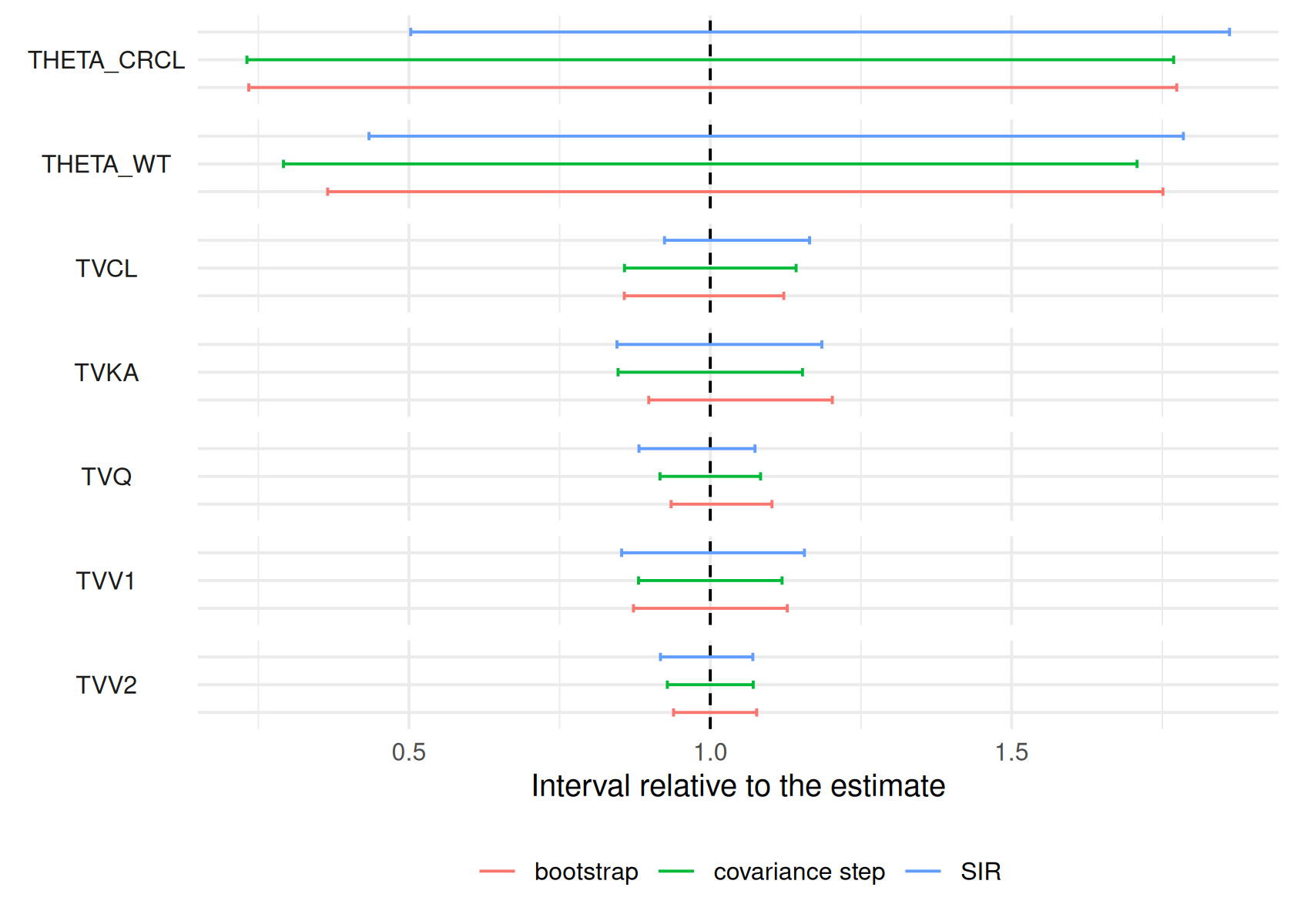

Figure 10.2: 95% intervals for the fixed effects from the covariance step, SIR and the bootstrap (percentile).

The structural parameters are precisely estimated by every route. The covariate exponents THETA_WT and THETA_CRCL have wide intervals, and the three routes differ in how wide. For a small dataset like this one, report the method you used and, where it matters, check that the conclusions hold under a second method.

Pitfalls

An unreliable covariance step. A fit can report standard errors that should not be trusted. The fit from NCA-based starting values in Initial estimates and a first fit is an example: its covariance matrix had to be regularised.

base <- ferx_example("two_cpt_oral_base")
fit_bad <- ferx_fit(base$model, base$data, inits_from_nca = TRUE, verbose = FALSE)
w_bad <- ferx_get_warnings(fit_bad, as_df = TRUE)
w_bad[w_bad$category %in% c("covariance_regularized", "condition_number"), c("severity", "category")]
#>   severity               category
#> 3  warning covariance_regularized
#> 7 critical       condition_number

In such a case, fix the model before quantifying uncertainty. covariance_fallback = "sir" runs SIR automatically when the covariance step fails.

Other points:

ferx_sir() and ferx_covariance() check that the model and data files are unchanged since the fit, and stop otherwise.
A bootstrap is samples complete fits. Set directory for long runs, so an interrupted run can be resumed and re-summarised.
Bayesian intervals require converged chains. Check fit$bayes$rhat and the effective sample sizes.

Warnings you may see here

See convergence and covariance warnings and resampling warnings.

covariance_step (info): a note on the covariance step, for example its cost.
covariance_failed (critical): the covariance step failed and there are no standard errors. Use covariance_fallback = "sir" or refit with different starting values.
covariance_regularized (warning): the step succeeded but was regularised, so the standard errors may be optimistic. Inspect the eigenvalues or use SIR or bootstrap intervals.
sir (warning): SIR failed or was requested without a covariance matrix, or its proposal did not cover some directions (named in the message).

Summary

The covariance step gives asymptotic standard errors in fit$estimates. ferx_covariance() reruns it with another estimator.
ferx_sir() (or sir = TRUE) gives resampling intervals. Check sir_ess.
ferx_bootstrap() refits resampled datasets. ferx_bootstrap_summarize() and plot() work on its results.
Compare routes for poorly determined parameters such as covariate effects.

Next: Simulating scenarios simulates scenarios with the final model, including parameter uncertainty.

Reference

R help: ?ferx_covariance, ?ferx_sir, ?ferx_bootstrap, ?ferx_bootstrap_summarize, ?plot.ferx_bootstrap
ferx-core: covariance and standard errors, SIR, bootstrap