Binary endpoints

Where you are

Some endpoints are yes/no outcomes: a response, an adverse event, a seizure-free day. ferx models them with a [binary_model] block: the log-odds of the outcome is an expression of parameters, random effects, covariates and time, and the likelihood is Bernoulli. This chapter fits the bundled logistic example, checks it against ordinary logistic regression in R, adds a random effect, and checks the model by simulation.

Maturity

Binary endpoints are the first of ferx-core’s categorical endpoints. Ordinal, count and other link functions are planned, not available. See the ferx-core categorical endpoints page.

The data

binary_logistic has 60 subjects with an outcome at times 0, 1 and 2, and a subject covariate X. DV is the 0/1 outcome on CMT = 3. There are no dose records:

binary <- ferx_example("binary_logistic")
binary_dir <- book_tempdir("binary")
binary_data <- read.csv(binary$data, na.strings = ".")
head(binary_data, 6)
#>   ID TIME DV CMT EVID MDV       X
#> 1  1    0  0   3    0   0  1.0692
#> 2  1    1  0   3    0   0  1.0692
#> 3  1    2  1   3    0   0  1.0692
#> 4  2    0  0   3    0   0 -1.0085
#> 5  2    1  0   3    0   0 -1.0085
#> 6  2    2  1   3    0   0 -1.0085
binary_data |> group_by(TIME) |> summarise(subjects = n(), fraction_1 = mean(DV))
#> # A tibble: 3 × 3
#>    TIME subjects fraction_1
#>   <int>    <int>      <dbl>
#> 1     0       60       0.35
#> 2     1       60       0.55
#> 3     2       60       0.7

Minimal runnable call

A logistic model needs only [parameters], [binary_model] and [fit_options]. cmt names the endpoint’s CMT value, and logit is the log-odds of DV = 1:

invisible(ferx_model_get_section(binary$model, "parameters"))
#> # [parameters]
#>   theta TH0(0.0, -10.0, 10.0)
#>   theta THX(0.0, -10.0, 10.0)
#>   theta THT(0.0, -10.0, 10.0)
invisible(ferx_model_get_section(binary$model, "binary_model"))
#> # [binary_model]
#>   cmt   = 3
#>   logit = TH0 + THX * X + THT * TIME
fit_binary <- ferx_fit(binary$model, binary$data, verbose = FALSE)
fit_binary$estimates[, c("estimate", "se", "rse_pct")]
#>       estimate        se  rse_pct
#> TH0 -0.7748495 0.2665858 34.40485
#> THX  0.8709007 0.2091270 24.01273
#> THT  0.8268374 0.2107385 25.48730
fit_binary$ofv
#> [1] 213.5955

Reading the result

Without random effects this is ordinary logistic regression. R’s glm() gives the same estimates and standard errors, and its residual deviance equals the OFV, which ferx reports on the −2 log-likelihood scale:

reference <- glm(DV ~ X + TIME, family = binomial, data = binary_data)
data.frame(ferx = fit_binary$theta, glm = coef(reference),
           ferx_se = fit_binary$estimates$se, glm_se = sqrt(diag(vcov(reference))))
#>           ferx        glm   ferx_se    glm_se
#> TH0 -0.7748495 -0.7751720 0.2665858 0.2665817
#> THX  0.8709007  0.8701400 0.2091270 0.2090772
#> THT  0.8268374  0.8270292 0.2107385 0.2107273
c(ferx_ofv = fit_binary$ofv, glm_deviance = reference$deviance)
#>     ferx_ofv glm_deviance 
#>     213.5955     213.5955

In sdtab, PRED and IPRED are probabilities of DV = 1 (typical and individual), IWRES is the Pearson residual (y − p) / √(p(1 − p)), and CWRES is not defined. There are no doses, so TAD and TAFD are empty:

head(fit_binary$sdtab, 4)
#>   ID TIME DV CMT      PRED     IPRED CWRES      IWRES  EBE_OFV N_OBS TAFD TAD
#> 1  1    0  0   3 0.5390000 0.5390000   NaN -1.0812943 4.453797   NaN  NaN NaN
#> 2  1    1  0   3 0.7277338 0.7277338   NaN -1.6348932 4.453797   NaN  NaN NaN
#> 3  1    2  1   3 0.8593610 0.8593610   NaN  0.4045434 4.453797   NaN  NaN NaN
#> 4  2    0  0   3 0.1606833 0.1606833   NaN -0.4375447 2.462139   NaN  NaN NaN

ferx_predict() returns concentration-type predictions and has no rows for a binary endpoint. The probabilities are in sdtab and in simulations:

nrow(ferx_predict(binary$model, binary$data, fit = fit_binary))
#> [1] 0

Options that matter

Key in `[binary_model]`	Meaning
`cmt`	The `CMT` value of this endpoint’s observation rows
`logit`	Log-odds of `DV = 1`: any expression of thetas, etas, covariates, individual parameters and `TIME`
`link`	Optional; `logit` is the only link available

Observation rows carry DV 0 or 1 and EVID = 0. Any other value stops the fit.
Covariates enter at their subject value; a covariate column that changes over time is not yet supported in logit (use TIME for time effects).
FOCEI, SAEM and IMP are suitable estimation methods (categorical estimation).

Variants

A random intercept

Subjects may differ in their tendency to respond. A random intercept ETA_I in the log-odds makes the model a mixed-effects logistic regression:

ri_lines <- readLines(binary$model)
ri_lines <- append(ri_lines, "  omega ETA_I ~ 0.5", after = grep("theta THT", ri_lines))
ri_lines <- sub("logit = TH0 + THX * X + THT * TIME", "logit = TH0 + THX * X + THT * TIME + ETA_I", ri_lines, fixed = TRUE)
ri_model <- file.path(binary_dir, "binary_random_intercept.ferx")
writeLines(ri_lines, ri_model)
invisible(ferx_model_get_section(ri_model, "binary_model"))
#> # [binary_model]
#>   cmt   = 3
#>   logit = TH0 + THX * X + THT * TIME + ETA_I
fit_ri <- ferx_fit(ri_model, binary$data, verbose = FALSE)
fit_ri$estimates[, c("estimate", "rse_pct")]
#>         estimate   rse_pct
#> TH0   -0.8501256  35.62861
#> THX    0.9504550  26.92926
#> THT    0.8999345  26.04293
#> ETA_I  0.4079273 116.36197
c(without_random_effect = fit_binary$ofv, with_random_effect = fit_ri$ofv)
#> without_random_effect    with_random_effect 
#>              213.5955              212.4832

With three outcomes per subject, the variance of the random intercept is poorly determined (relative standard error above 100%), and its shrinkage is high (56%). The OFV drops by only 1.11 for one extra parameter: these data do not support between-subject variability in the response.

SAEM, which avoids the Laplace approximation, is an alternative for sparse binary data. On this weakly informative model its result depends on the random seed. Seeds 1 to 3 agree with each other and with FOCEI; the run with the engine’s default seed ends elsewhere, with a regularized covariance step:

saem_seeds <- list(default = NULL, seed_1 = list(seed = 1), seed_2 = list(seed = 2), seed_3 = list(seed = 3))
do.call(rbind, lapply(names(saem_seeds), function(name) {
  # suppress the R warning that reports overriding the model file's method
  f <- suppressWarnings(ferx_fit(ri_model, binary$data, method = "saem", settings = saem_seeds[[name]],
                                 verbose = FALSE))
  data.frame(run = name, ofv = f$ofv, t(setNames(f$estimates$estimate, rownames(f$estimates))),
             max_rse_pct = max(f$estimates$rse_pct),
             covariance_regularized = "covariance_regularized" %in% ferx_get_warnings(f, as_df = TRUE)$category)
}))
#>       run      ofv        TH0       THX       THT     ETA_I  max_rse_pct
#> 1 default 212.8381 -0.7809784 0.8912139 0.8331141 0.1603772 2284772.9988
#> 2  seed_1 212.5041 -0.8198987 0.9468319 0.8736665 0.3574003     132.1920
#> 3  seed_2 212.5060 -0.8117019 0.9284252 0.8685714 0.3831907     118.0836
#> 4  seed_3 212.5119 -0.8031152 0.9331072 0.8647746 0.3702206     127.6059
#>   covariance_regularized
#> 1                   TRUE
#> 2                  FALSE
#> 3                  FALSE
#> 4                  FALSE

Set the seed for SAEM fits, and compare a few seeds when a variance is weakly identified (Estimation methods and controlling the fit).

Checking the model by simulation

ferx_simulate() draws a new 0/1 outcome for each observation record from the fitted probability. Comparing the observed fraction of ones with the simulated fractions is the binary counterpart of a visual predictive check (Simulation-based evaluation: VPC). Here it is split by time and by the sign of X:

simulated <- ferx_simulate(binary$model, binary$data, n_sim = 500, seed = 1, fit = fit_binary)
groups <- distinct(binary_data, ID, X) |> mutate(group = ifelse(X > 0, "X > 0", "X <= 0"))
simulated_fraction <- simulated |>
  mutate(ID = as.integer(ID)) |>
  left_join(groups, by = "ID") |>
  group_by(SIM, TIME, group) |>
  summarise(fraction = mean(DV_SIM), .groups = "drop") |>
  group_by(TIME, group) |>
  summarise(lo = quantile(fraction, 0.05), hi = quantile(fraction, 0.95), .groups = "drop")
observed_fraction <- binary_data |>
  left_join(groups, by = c("ID", "X")) |>
  group_by(TIME, group) |>
  summarise(fraction = mean(DV), .groups = "drop")
ggplot(simulated_fraction, aes(TIME)) +
  geom_errorbar(aes(ymin = lo, ymax = hi), width = 0.1) +
  geom_point(data = observed_fraction, aes(y = fraction), colour = "steelblue", size = 2.5) +
  facet_wrap(~ group) +
  labs(x = "Time", y = "Fraction with DV = 1")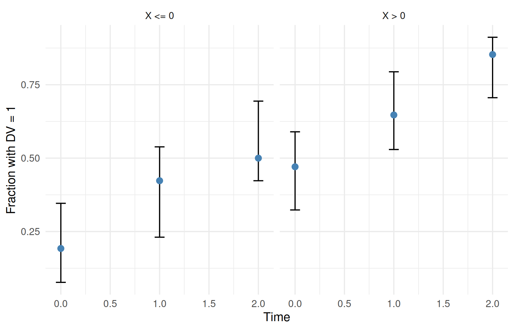

Figure 21.1: Observed fraction of ones (points) and the 90% interval of 500 simulated fractions (bars), by time and covariate group.

Binary endpoints with a PK model

logit can use individual parameters from [individual_parameters], so a binary endpoint can be combined with other model parts. No bundled example links a binary outcome to a PK model; see the ferx-core categorical endpoints page for the namespace logit can read. The related [markov_model] block for transitions between states is listed in Function, option and example index.

Pitfalls

DV must be 0 or 1. An outcome with more categories stops the fit:

bad_data <- binary_data
bad_data$DV[1] <- 2
bad_file <- file.path(binary_dir, "binary_dv2.csv")
write.csv(bad_data, bad_file, row.names = FALSE)
try(ferx_fit(binary$model, bad_file, verbose = FALSE))
#> Error in ferx_rust_fit(model_path = normalizePath(model), data_path = normalizePath(data),  : 
#>   Fit error: [binary_model] cmt = 3: observed DV must be 0 or 1 (Bernoulli), got 2. For an ordered response with more than two categories use an ordinal endpoint (not yet supported).

Few outcomes per subject carry little information on random effects. Check shrinkage and the OFV change before keeping a random effect.
Use sdtab or simulations for probabilities, not ferx_predict().
print() on a binary fit summarises the model with labels meant for concentration models. Read the estimates from fit$estimates.

Warnings you may see here

data_quality (warning): here it reports that the subjects use finite-difference inner gradients. That is expected for a binary endpoint, and the results are correct.

Summary

Declare a binary endpoint with [binary_model]: cmt and a logit expression.
Without random effects the fit equals logistic regression; the OFV is the deviance.
Add random effects to the log-odds for a mixed-effects model, and check whether the data support them.
sdtab holds probabilities and Pearson residuals; simulations give 0/1 outcomes for predictive checks.

Next: Time-to-event models models times to events.

Reference

R help: ?ferx_fit, ?ferx_simulate
ferx-core: categorical endpoints, categorical estimation