Dosing regimens and exposure metrics

Where you are

Most earlier chapters used a single dose per subject. Real studies repeat doses, sample at steady state, infuse, or give doses into absorption processes. This chapter shows how these regimens are written in the dataset, and how ferx computes exposure metrics per subject and per dosing interval with [derived].

Maturity

The dataset columns used here are part of the stable ferx data format. [derived] and the built-in absorption models are beta in ferx-core. See feature maturity.

The data

In warfarin_addl, each subject has a single dose record that stands for seven daily doses: II = 24 is the interval and ADDL = 6 the number of additional doses. Samples are taken on days 1, 2, 4, 6, 7 and 8:

addl <- ferx_example("warfarin_addl")
dosing_dir <- book_tempdir("dosing")
addl_data <- read.csv(addl$data, na.strings = ".")
filter(addl_data, ID == 1) |> select(ID, TIME, DV, EVID, AMT, II, ADDL)
#>    ID  TIME      DV EVID AMT II ADDL
#> 1   1   0.0      NA    1 100 24    6
#> 2   1   0.5  4.8991    0  NA  0    0
#> 3   1   1.0  8.6395    0  NA  0    0
#> 4   1   2.0  7.4206    0  NA  0    0
#> 5   1   4.0 10.4268    0  NA  0    0
#> 6   1   8.0  7.6090    0  NA  0    0
#> 7   1  24.0  6.3220    0  NA  0    0
#> 8   1  28.0 10.0212    0  NA  0    0
#> 9   1  32.0 11.3024    0  NA  0    0
#> 10  1  72.0  9.5836    0  NA  0    0
#> 11  1 120.0 12.4406    0  NA  0    0
#> 12  1 144.0 15.4449    0  NA  0    0
#> 13  1 145.0 20.7495    0  NA  0    0
#> 14  1 146.0 28.5110    0  NA  0    0
#> 15  1 148.0 23.8443    0  NA  0    0
#> 16  1 152.0 20.4556    0  NA  0    0
#> 17  1 168.0 10.8486    0  NA  0    0

Minimal runnable call: repeated doses

A dataset with ADDL fits like any other:

fit_addl <- ferx_fit(addl$model, addl$data, verbose = FALSE)
fit_addl$theta
#>      TVCL       TVV      TVKA 
#>  0.220865 10.594506  1.668516

ferx expands the record into seven doses before fitting. Writing the seven dose rows out explicitly gives the same fit:

dose_rows <- filter(addl_data, EVID == 1)
explicit_doses <- dose_rows[rep(seq_len(nrow(dose_rows)), dose_rows$ADDL + 1), ] |>
  group_by(ID) |>
  mutate(TIME = TIME + (row_number() - 1) * II, II = 0, ADDL = 0) |>
  ungroup()
explicit <- bind_rows(explicit_doses, filter(addl_data, EVID == 0)) |> arrange(ID, TIME, desc(EVID))
explicit_file <- file.path(dosing_dir, "warfarin_explicit_doses.csv")
write.csv(explicit, explicit_file, row.names = FALSE, na = ".")
c(addl = fit_addl$ofv, explicit_rows = ferx_fit(addl$model, explicit_file, verbose = FALSE)$ofv)
#>          addl explicit_rows 
#>      437.3381      437.3381

Reading the result: time after dose and exposure per subject

sdtab has two time columns besides TIME: TAFD, the time after the first dose, and TAD, the time after the most recent dose, which restarts at each expanded dose. The model’s [derived] block uses them for exposure metrics:

invisible(ferx_model_get_section(addl$model, "derived"))
#> # [derived]
#>   KE     = CL / V
#>   T_HALF = 0.6931472 / KE
#> 
#>   # TAFD uses the first dose time; TAD resets at each expanded dose
#>   DAY    = floor(TAFD / 24) + 1
#> 
#>   CMAX   = max(IPRED)
#> 
#>   # Trough: minimum IPRED at dose time (TAD ~= 0 after ADDL expansion).
#>   # 1e-10 absorbs floating-point residuals from modular arithmetic.
#>   CMIN_TAU = min(IPRED, TAD < 1e-10)
#> 
#>   # Trough via window: last 4 h of the interval (no precision concern)
#>   CMIN_LATE = min(IPRED, TAD > 20)
#> 
#>   AUC_TAU = integral(IPRED, window=24, anchor=0, step=0.1)
fit_addl$sdtab |>
  filter(ID == 1) |>
  select(TIME, TAFD, TAD, DAY, IPRED, CMAX, CMIN_TAU, CMIN_LATE)
#>     TIME  TAFD  TAD DAY     IPRED     CMAX CMIN_TAU CMIN_LATE
#> 1    0.5   0.5  0.5   1  5.250084 21.80407 5.690902  13.92952
#> 2    1.0   1.0  1.0   1  7.467992 21.80407 5.690902  13.92952
#> 3    2.0   2.0  2.0   1  8.712081 21.80407 5.690902  13.92952
#> 4    4.0   4.0  4.0   1  8.658896 21.80407 5.690902  13.92952
#> 5    8.0   8.0  8.0   1  7.970254 21.80407 5.690902  13.92952
#> 6   24.0  24.0  0.0   2  5.690902 21.80407 5.690902  13.92952
#> 7   28.0  28.0  4.0   2 13.890178 21.80407 5.690902  13.92952
#> 8   32.0  32.0  8.0   2 12.779037 21.80407 5.690902  13.92952
#> 9   72.0  72.0  0.0   4 11.196053 21.80407 5.690902  13.92952
#> 10 120.0 120.0  0.0   6 13.200035 21.80407 5.690902  13.92952
#> 11 144.0 144.0  0.0   7 13.655015 21.80407 5.690902  13.92952
#> 12 145.0 145.0  1.0   7 20.838532 21.80407 5.690902  13.92952
#> 13 146.0 146.0  2.0   7 21.804073 21.80407 5.690902  13.92952
#> 14 148.0 148.0  4.0   7 21.211078 21.80407 5.690902  13.92952
#> 15 152.0 152.0  8.0   7 19.508672 21.80407 5.690902  13.92952
#> 16 168.0 168.0 24.0   8 13.929523 21.80407 5.690902  13.92952

CMAX and the two troughs have one value per subject. CMIN_TAU filters on TAD < 1e-10, the samples taken at dose times (24, 72, 120 and 144 hours; the tolerance absorbs rounding). CMIN_LATE filters on the last 4 hours of an interval, which here only the sample at 168 hours meets.

The typical profile over the whole regimen comes from ferx_predict() on a design with the same dose record and a fine time grid. The W_DESIGN_DV warning is the expected one for a design file with empty DV cells (Simulating scenarios):

design <- data.frame(ID = 1, TIME = c(0, seq(0.25, 192, by = 0.25)), DV = NA,
                     EVID = c(1, rep(0, 768)), AMT = c(100, rep(NA, 768)), CMT = 1, RATE = 0,
                     MDV = c(1, rep(0, 768)), II = c(24, rep(0, 768)), ADDL = c(6, rep(0, 768)))
design_file <- file.path(dosing_dir, "addl_design.csv")
write.csv(design, design_file, row.names = FALSE, na = ".")
typical <- ferx_predict(addl$model, design_file, fit = fit_addl)
#> Warning: ferx_predict produced 1 diagnostic:
#>   W_DESIGN_DV: 768 observation row(s) (EVID=0) had a missing DV (`.`/`NA`/blank) and were kept as design points to simulate at. A fit of the same dataset would skip these rows (W_MISSING_DV), so the simulated dataset has more rows than the fitted one. Set MDV=1 on rows that are not sampling times.
ggplot(typical, aes(TIME, PRED)) +
  geom_line() +
  geom_point(data = filter(addl_data, EVID == 0), aes(TIME, DV), alpha = 0.4) +
  geom_vline(xintercept = seq(0, 144, by = 24), linetype = "dotted") +
  labs(x = "Time (h)", y = "Concentration")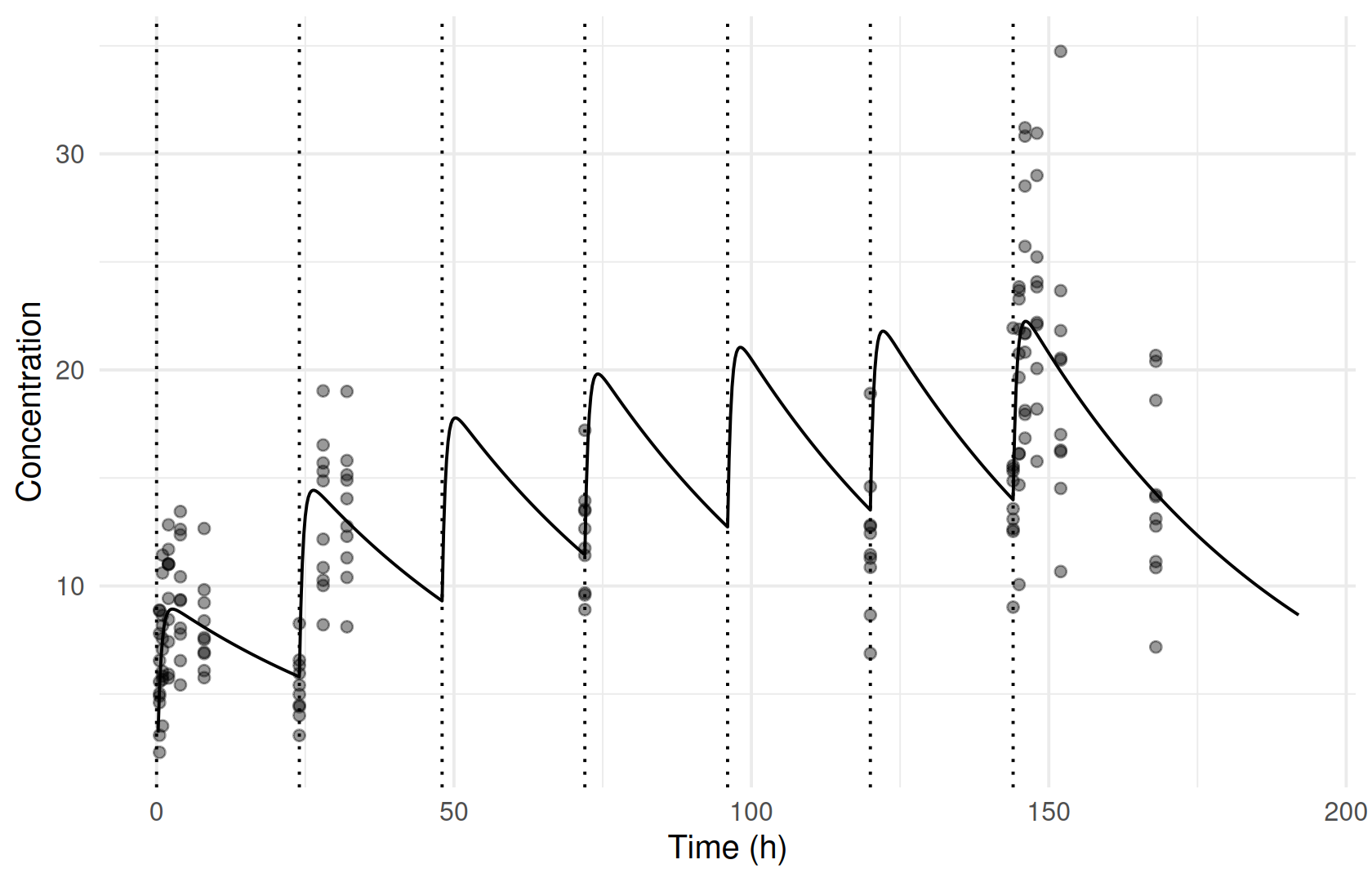

Figure 18.1: Typical concentration profile over seven daily doses (line) with the observed concentrations (points).

Options that matter

Dose records use these columns of the ferx data format (Preparing and checking the analysis dataset):

Column	Meaning
`EVID`	`1` for a dose; `2` other event, `3` reset, `4` reset and dose
`AMT`, `CMT`	Amount and the compartment it goes into
`RATE`	`0` for a bolus; a positive rate for a zero-order input over `AMT / RATE`
`II`, `ADDL`	Interval and number of additional doses after this one
`SS`	`1`: the dose is the last of an infinite series at interval `II` (steady state)

Time quantities available in [derived] and in [odes]:

Name	Meaning
`TIME`	Time in the dataset
`TAFD`	Time after the first dose
`TAD`	Time after the most recent dose (steady-state aware)

[derived] aggregates and integrals for exposure metrics, with the filters used in this chapter:

Expression	Result
`max(IPRED)`, `tmax(IPRED)`, `min(IPRED)`	One value per subject over the observation rows
`min(IPRED, TAD < 1e-10)`	The same, over the rows where the filter holds (`NaN` if none)
`integral(IPRED, from=0, to=72)`	Area over a fixed interval
`integral(X, window=24, anchor=0, step=0.1)`	One area per dosing window
`integral(DV, from=0, to=72)`	Area of the observations, at the observation times

The ferx-core data format and [derived] pages give the full rules.

Variants

Steady state

warfarin_ss samples one dosing interval of a once-daily regimen at steady state. The dose record carries SS = 1 and II = 24, and the concentrations are higher than after a single dose:

ss <- ferx_example("warfarin_ss")
ss_data <- read.csv(ss$data, na.strings = ".")
filter(ss_data, ID == 1)
#>   ID TIME      DV EVID AMT CMT RATE MDV SS II
#> 1  1  0.0      NA    1 100   1    0   1  1 24
#> 2  1  0.5 23.3448    0  NA   1    0   0  0  0
#> 3  1  1.0 25.9891    0  NA   1    0   0  0  0
#> 4  1  2.0 26.7357    0  NA   1    0   0  0  0
#> 5  1  4.0 30.6482    0  NA   1    0   0  0  0
#> 6  1  8.0 23.8695    0  NA   1    0   0  0  0
#> 7  1 12.0 26.1273    0  NA   1    0   0  0  0
#> 8  1 24.0 15.8599    0  NA   1    0   0  0  0
fit_ss <- ferx_fit(ss$model, ss$data, verbose = FALSE)
fit_ss$theta
#>     TVCL      TVV     TVKA 
#> 0.153102 8.963594 1.611488

An SS = 1 dose stands for an infinite series of earlier doses. A long explicit run-in gives the same predictions. Here 30 daily doses precede the sampled interval:

run_in <- ss_data |>
  mutate(TIME = ifelse(EVID == 0, TIME + 30 * 24, TIME), SS = 0, ADDL = ifelse(EVID == 1, 30, 0))
run_in_file <- file.path(dosing_dir, "warfarin_run_in.csv")
write.csv(run_in, run_in_file, row.names = FALSE, na = ".")
steady <- ferx_predict(ss$model, ss$data, fit = fit_ss)
explicit_run_in <- ferx_predict(ss$model, run_in_file, fit = fit_ss)
head(data.frame(TIME = steady$TIME, steady_state = steady$PRED, run_in = explicit_run_in$PRED), 7)
#>   TIME steady_state   run_in
#> 1  0.5     28.20589 28.20579
#> 2  1.0     30.71017 30.71007
#> 3  2.0     31.95331 31.95321
#> 4  4.0     31.29640 31.29631
#> 5  8.0     29.24627 29.24618
#> 6 12.0     27.31487 27.31479
#> 7 24.0     22.25276 22.25270
max(abs(steady$PRED / explicit_run_in$PRED - 1))
#> [1] 0.000003568003

Exposure per dosing window

AUC_TAU = integral(IPRED, window=24, anchor=0, step=0.1) gives one area per 24-hour window. With IPRED, the values on the fine grid are taken from the nearest observation, so the result depends on the sampling (Model states in [derived]). An integral over the model state, compartments[1] (the central concentration in this analytical model), evaluates the model on the grid instead. The comparison below adds that column and computes the exact area of each window for subject 1 from its individual parameters:

Table 18.1: Area per 24-hour window for subject 1: from IPRED, from the model state, and exact.

state_lines <- sub("AUC_TAU = integral(IPRED, window=24, anchor=0, step=0.1)",
                   "AUC_TAU = integral(IPRED, window=24, anchor=0, step=0.1)\n  AUC_TAU_STATE = integral(compartments[1], window=24, anchor=0, step=0.1)",
                   readLines(addl$model), fixed = TRUE)
state_model <- file.path(dosing_dir, "warfarin_addl_state_auc.ferx")
writeLines(state_lines, state_model)
fit_state <- ferx_fit(state_model, addl$data, verbose = FALSE)

p <- filter(fit_state$individual_estimates, ID == "1")
ke <- p$CL / p$V
concentration <- function(t) {
  sapply(t, function(time) sum(sapply(seq(0, 144, by = 24), function(dose_time) {
    tad <- time - dose_time
    if (tad <= 0) 0 else 100 * p$KA / (p$V * (p$KA - ke)) * (exp(-ke * tad) - exp(-p$KA * tad))
  })))
}
distinct(filter(fit_state$sdtab, ID == 1), DAY, AUC_TAU, AUC_TAU_STATE) |>
  mutate(AUC_EXACT = sapply(DAY, function(day) integrate(concentration, (day - 1) * 24, day * 24)$value))
#>   DAY  AUC_TAU AUC_TAU_STATE AUC_EXACT
#> 1   1 173.9020      172.0675  172.0806
#> 2   2 296.6108      279.2894  279.3025
#> 3   4 268.7053      383.0116  383.0247
#> 4   6 322.2378      420.7686  420.7816
#> 5   7 430.5146      429.3408  429.3538
#> 6   8 334.3086      262.4453  262.4452

The state integral matches the exact areas and rises as the drug accumulates. The IPRED integral does not: the day-4 window, with a single sample, even comes out below day 2. Windows are reported on the rows that fall in them, so days 3 and 5, which have no samples, have no row.

Filters without matching rows

warfarin_derived defines metrics for a multiple-dose study, but ships with the single-dose warfarin data. Aggregates whose filter matches no row are NaN: there is no sample at a dose time (CTROUGH) and none on day 14 (CMAX_D14). On the seven-dose data the trough is defined, and day 14 is still outside the study:

derived <- ferx_example("warfarin_derived")
invisible(ferx_model_get_section(derived$model, "derived"))
#> # [derived]
#>   # Per-row: elimination rate and half-life
#>   KE     = CL / V
#>   T_HALF = 0.6931472 / KE
#> 
#>   # Which dosing day (tau = 24 h)
#>   DAY      = floor(TAFD / 24) + 1
#>   TAU_TIME = TAFD mod 24
#> 
#>   # Subject-level aggregates (one scalar per subject, repeated across rows)
#>   CMAX       = max(IPRED)
#>   TMAX       = tmax(IPRED)
#>   # 1e-10 absorbs floating-point residuals when TAD is mathematically 0
#>   CTROUGH    = min(IPRED, TAD < 1e-10)
#>   CMAX_D1    = max(IPRED, TAFD < 24)
#>   CMAX_D14   = max(IPRED, TAFD >= 312 && TAFD < 336)
#> 
#>   # AUC over first 72 h (fine internal grid, 500 steps)
#>   AUC_0_72   = integral(IPRED, from=0, to=72)
#> 
#>   # Periodic AUC: one value per 24-h dosing window
#>   AUC_TAU    = integral(IPRED, window=24, anchor=0, step=0.1)
#> 
#>   # DV-based AUC (observation times only -- no interpolation)
#>   AUC_DV_72  = integral(DV, from=0, to=72)
fit_single <- ferx_fit(derived$model, derived$data, verbose = FALSE)
fit_repeated <- ferx_fit(derived$model, addl$data, verbose = FALSE)
metrics <- c("CMAX", "TMAX", "CTROUGH", "CMAX_D1", "CMAX_D14", "AUC_0_72", "AUC_DV_72")
bind_rows(single_dose = distinct(filter(fit_single$sdtab, ID == 1), across(all_of(metrics))),
          seven_doses = distinct(filter(fit_repeated$sdtab, ID == 1), across(all_of(metrics))), .id = "data")
#>          data     CMAX TMAX  CTROUGH   CMAX_D1 CMAX_D14 AUC_0_72 AUC_DV_72
#> 1 single_dose 11.38329    4      NaN 11.383285      NaN 510.6520  506.8519
#> 2 seven_doses 21.80407  146 5.690902  8.712081      NaN 745.9969  669.8353

AUC_DV_72 integrates the observations at their sampling times, so it is lower than the model-based area when sampling is sparse.

Doses into absorption processes

A dose into a compartment fed by a built-in absorption function (Absorption and bioavailability) can be a steady-state dose or an infusion. The dose then passes through the absorption process. ss_absorption gives an SS = 1 dose every 8 hours into first_order(ka=KA), and infusion_absorption infuses 100 at a rate of 25 into the same kind of model. Both are single-subject prediction examples:

ss_abs <- ferx_example("ss_absorption")
inf_abs <- ferx_example("infusion_absorption")
grep("d/dt", readLines(ss_abs$model), value = TRUE)
#> [1] "  d/dt(central) = first_order(ka=KA) - CL/V*central"
read.csv(ss_abs$data, na.strings = ".")[1:2, ]
#>   ID TIME     DV EVID AMT CMT MDV II SS
#> 1  1  0.0     NA    1 100   1   1  8  1
#> 2  1  0.5 12.231    0   0   1   0  0  0
read.csv(inf_abs$data, na.strings = ".")[1:2, ]
#>   ID TIME      DV EVID AMT CMT RATE MDV
#> 1  1    0      NA    1 100   1   25   1
#> 2  1    1 0.30468    0   0   1    0   0

A single first-order absorption route is also the analytical pk one_cpt_oral model, with the dose in its depot. Predicting both data files with that model gives the same concentrations. For the steady-state case, an explicit run-in of 60 doses does too:

analytical <- function(ka, file) {
  writeLines(c("[parameters]", "  theta TVCL(1.0, 0.01, 50.0)", "  theta TVV(20.0, 0.5, 200.0)",
               sprintf("  theta TVKA(%s, 0.005, 20.0)", ka), "  omega ETA_CL ~ 0.0 FIX",
               "  sigma PROP_ERR ~ 0.01 (sd)", "", "[individual_parameters]", "  CL = TVCL * exp(ETA_CL)",
               "  V  = TVV", "  KA = TVKA", "", "[structural_model]", "  pk one_cpt_oral(cl=CL, v=V, ka=KA)", "",
               "[error_model]", "  DV ~ proportional(PROP_ERR)"), file)
  file
}
ss_run_in <- read.csv(ss_abs$data, na.strings = ".") |>
  mutate(TIME = ifelse(EVID == 0, TIME + 60 * 8, TIME), SS = 0, ADDL = ifelse(EVID == 1, 60, 0))
ss_run_in_file <- file.path(dosing_dir, "ss_absorption_run_in.csv")
write.csv(ss_run_in, ss_run_in_file, row.names = FALSE, na = ".")

data.frame(TIME = ferx_predict(ss_abs$model, ss_abs$data)$TIME,
           steady_state_kernel = ferx_predict(ss_abs$model, ss_abs$data)$PRED,
           analytical = ferx_predict(analytical(0.15, file.path(dosing_dir, "ss_analytical.ferx")), ss_abs$data)$PRED,
           run_in_60_doses = ferx_predict(ss_abs$model, ss_run_in_file)$PRED)
#>   TIME steady_state_kernel analytical run_in_60_doses
#> 1  0.5            12.23056   12.23056        12.23056
#> 2  1.0            12.40221   12.40221        12.40221
#> 3  2.0            12.63355   12.63355        12.63355
#> 4  4.0            12.73541   12.73541        12.73541
#> 5  6.0            12.48957   12.48957        12.48957
#> 6  7.9            12.04432   12.04432        12.04432
data.frame(TIME = ferx_predict(inf_abs$model, inf_abs$data)$TIME,
           infusion_kernel = ferx_predict(inf_abs$model, inf_abs$data)$PRED,
           analytical = ferx_predict(analytical(0.6, file.path(dosing_dir, "inf_analytical.ferx")), inf_abs$data)$PRED)
#>   TIME infusion_kernel analytical
#> 1    1       0.3046785  0.3046785
#> 2    2       1.0071482  1.0071482
#> 3    4       2.8771566  2.8771566
#> 4    6       3.8508179  3.8508179
#> 5   10       3.6059222  3.6059222

The two examples declare omega ETA_CL ~ 0.0 without FIX. That is fine for prediction, but a fit stops and asks for FIX or a positive starting variance (Variability: random effects, residual error and IOV):

fit_attempt <- tryCatch(ferx_fit(ss_abs$model, ss_abs$data, verbose = FALSE), error = conditionMessage)
sub(",.*", "", fit_attempt)  # first clause
#> [1] "Fit error: `omega ETA_CL ~ 0.0` declares no variability but is not `FIX`-ed"

Other dose records

Infusions into the central compartment: RATE > 0 on a dose into a compartment without an absorption process. No bundled ferx-r example uses a fixed-rate infusion into the central compartment. See the ferx-core data format page.
Other events and resets: EVID = 2 records carry covariate changes or output times without a dose. EVID = 3 resets the system, and EVID = 4 resets and doses, for example between study periods. No bundled example uses them.
Designs for simulation: dose records with II and ADDL in a design dataset, as in Simulating scenarios.

Pitfalls

Aggregates and integrals use the observation rows. CMAX, troughs and IPRED integrals only see sampled times. Use integrals over model states, or predictions on a fine design, for model-based exposure.
A filter can match nothing. The metric is then NaN. Check the sampling design before reading a TAD- or day-based metric.
Test for a dose time with a tolerance. TAD < 1e-10 rather than TAD == 0.
Steady state needs II. An SS = 1 record uses II as the interval. For doses into built-in absorption processes, ferx-core rejects steady state combined with an absorption lag time or a zero_order() input (absorption).

Warnings you may see here

data_quality (warning): inconsistent ADDL/II records, or other dataset problems (Preparing and checking the analysis dataset).

Summary

II with ADDL writes repeated doses compactly; the fit is identical to explicit dose rows.
SS = 1 puts a dose at steady state; predictions match a long explicit run-in.
TAD and TAFD restart per dose and count from the first dose; use them in [derived] filters.
Integrate model states for exposure per dosing window. IPRED integrals depend on the sampling.
Steady-state doses and infusions pass through built-in absorption processes.

Next: Censored observations (BLOQ) handles concentrations below the limit of quantification.

Reference

R help: ?ferx_fit, ?ferx_predict
ferx-core: data format, [derived], absorption