Estimation methods and controlling the fit

Where you are

Initial estimates and a first fit fitted the base model with the method from its model file (FOCEI). ferx offers several estimation methods, and every method and optimizer can be tuned. This chapter shows how to choose a method, chain methods, follow what the optimizer does, and control the fit through settings. It ends with multi-start and background fits.

The data

The base model of the workflow thread, plus the smaller warfarin example for the method comparison:

base <- ferx_example("two_cpt_oral_base")
warf <- ferx_example("warfarin")

Estimation methods

method selects the estimator:

`method`	Estimator	Notes
`"foce"`	First-order conditional estimation
`"focei"`	FOCE with interaction	The default when neither the call nor the model file sets a method
`"laplace"`	Laplace approximation with the exact Hessian	Reports a different OFV than `"focei"`. With `n_agq > 1` it becomes adaptive Gauss-Hermite quadrature
`"gn"`, `"gn_hybrid"`	Gauss-Newton; the hybrid finishes with a FOCEI polish step
`"saem"`	Stochastic approximation EM	Stochastic: set `seed` for reproducibility
`"imp"`	Importance-sampling Monte Carlo EM	With `imp_eval_only = TRUE` it only evaluates −2 log L and must be the last chain stage
`"impmap"`	Importance sampling assisted by the mode a posteriori	Requires mu-referencing; no IOV yet
`"bayes"`	Full MCMC	Posterior summaries in `fit$bayes` instead of a covariance step
`vi` (model file only)	Variational inference	Set in `[fit_options]`; not accepted by the `method` argument (see below)

The ferx-core estimation methods pages describe each algorithm. The same warfarin model fitted with each method:

Table 6.1: Warfarin fitted with every estimation method.

methods <- c("foce", "focei", "laplace", "gn", "gn_hybrid", "saem", "imp", "impmap", "bayes")
method_fits <- lapply(methods, function(m) {
  start <- Sys.time()
  # suppress the R warnings that report overriding the model file's method
  f <- suppressWarnings(ferx_fit(warf$model, warf$data, method = m, verbose = FALSE))
  data.frame(method = m, converged = f$converged, ofv = round(f$ofv, 2),
             TVCL = signif(f$theta[["TVCL"]], 4),
             seconds = round(as.numeric(difftime(Sys.time(), start, units = "secs")), 1))
})
do.call(rbind, method_fits)
#>      method converged     ofv   TVCL seconds
#> 1      foce      TRUE -280.36 0.1330     0.2
#> 2     focei      TRUE -286.00 0.1327     0.1
#> 3   laplace      TRUE -285.97 0.1327     0.5
#> 4        gn      TRUE -280.36 0.1329     0.0
#> 5 gn_hybrid      TRUE -280.36 0.1330     0.3
#> 6      saem      TRUE -279.93 0.1327     0.1
#> 7       imp      TRUE -279.93 0.1327    63.7
#> 8    impmap      TRUE -279.93 0.1327     2.3
#> 9     bayes      TRUE -593.69 0.1329     0.7

The estimates are close, but OFVs are not comparable across methods. Each method computes the objective function under its own approximation. Compare OFVs only between fits made with the same method, as in Model development and selection.

Minimal runnable call

Pass method to override the model file. A character vector runs a chain: each stage starts from the previous stage’s estimates, and only the last stage produces the covariance step and diagnostics.

fit_chain <- ferx_fit(base$model, base$data, method = c("saem", "focei"), verbose = FALSE)
#> Warning: Model file [fit_options] sets `method = focei` but ferx_fit() argument
#> overrides it with `saem, focei`. The call-time value will be used.
fit_chain$method_chain
#> [1] "SAEM"  "FOCEI"
c(converged = fit_chain$converged, ofv = fit_chain$ofv)
#> converged       ofv 
#>     1.000 -1185.217

Reading the result

Following the optimizer

With optimizer_trace = TRUE ferx records one row per objective evaluation. ferx_trace() returns it as a data frame:

fit <- ferx_fit(base$model, base$data, optimizer_trace = TRUE, verbose = FALSE)
trace <- ferx_trace(fit)
dim(trace)
#> [1] 98 39
head(trace[, c("iter", "method", "ofv", "wall_ms", "grad_norm", "step_norm", "optimizer")])
#>   iter method         ofv wall_ms grad_norm step_norm optimizer
#> 1    1  focei -1171.88242       6        NA        NA    bobyqa
#> 2    2  focei -1060.52606      13        NA  0.500000    bobyqa
#> 3    3  focei   -68.00626      21        NA  0.707107    bobyqa
#> 4    4  focei -1005.78590      24        NA  0.707107    bobyqa
#> 5    5  focei  -991.99282      30        NA  0.707107    bobyqa
#> 6    6  focei -1132.81660      32        NA  0.707107    bobyqa

plot() on a fit draws the trace. By default (monotonic = TRUE) the OFV panel shows the running minimum for FOCE/FOCEI, because their traces include rejected line-search trial points. log_ofv = TRUE shifts the OFV by its minimum; despite the name, it is not a log transform:

plot(fit)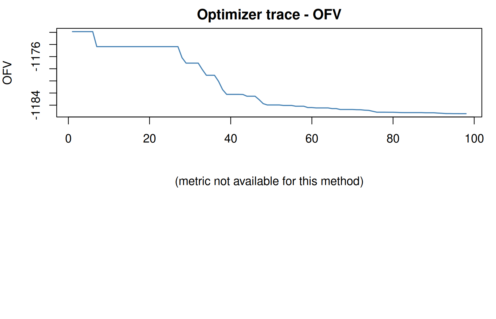

Figure 6.1: Optimizer trace of the base model fit.

Run logs

ferx_runlog() writes a plain-text record of the run: model file, data summary, estimates with initial values, settings, OFV, covariance diagnostics, shrinkage and runtime. With verbose = FALSE it returns the text instead of printing it, which is convenient for saving next to the results:

log_text <- ferx_runlog(fit, verbose = FALSE)
log_lines <- strsplit(log_text, "\n")[[1]]
start_line <- grep("PARAMETER ESTIMATES", log_lines)
cat(log_lines[(start_line - 1):(start_line + 14)], sep = "\n")
#> ============================================================
#> PARAMETER ESTIMATES
#> ------------------------------------------------------------
#>   PARAMETER                            INITIAL           FINAL        SE     %RSE
#>   --------------------------------------------------------------------------------
#>   TVCL                                       5         4.46476    0.3217     7.2%
#>   TVV1                                      50         48.2422     3.103     6.4%
#>   TVQ                                       10         9.58425     0.413     4.3%
#>   TVV2                                     100         93.7877     3.433     3.7%
#>   TVKA                                     1.2         1.24747   0.09754     7.8%
#>   ETA_CL                                   0.1        0.155125   0.04018    25.9%
#>   ETA_V1                                   0.1        0.119905   0.03256    27.2%
#>   ETA_Q                                   0.05       0.0525744   0.01445    27.5%
#>   ETA_V2                                  0.05       0.0384571   0.01051    27.3%
#>   ETA_KA                                  0.15        0.175835   0.04869    27.7%
#>   PROP_ERR                                0.02         0.01962  0.001123     5.7%

With a trace, show_iterations = TRUE (default) adds an iteration history, shortened to its first and last 10 rows for long runs. gradient_tol sets the relative-gradient threshold used in its convergence checks. ferx_runlog_iters() prints the full iteration history:

iters <- ferx_runlog_iters(fit, verbose = FALSE)
cat(head(strsplit(iters, "\n")[[1]], 10), sep = "\n")
#> ============================================================
#> ITERATION HISTORY
#> ------------------------------------------------------------
#>   ITER            OFV           dOFV    STEP_NORM
#>   ----  -------------  -------------  -----------
#>      1       -1171.88            ---           NA
#>      2       -1060.53       +111.356          0.5
#>      3       -68.0063        +992.52       0.7071
#>      4       -1005.79        -937.78       0.7071
#>      5       -991.993       +13.7931       0.7071

The gradient at the reported estimates

The run log’s convergence checks read fit$final_gradient, the gradient of the objective at the reported parameter point, in the packed space the optimizer works in (Variability: random effects, residual error and IOV). Gradient-based optimizers report the gradient they already used. The derivative-free bobyqa has none of its own, so ferx computes a central finite-difference gradient after the fit instead, which is what lets you check a converged = TRUE where it is least supported:

fit_bobyqa <- ferx_fit(warf$model, warf$data, settings = list(optimizer = "bobyqa"), verbose = FALSE)
data.frame(optimizer = fit_bobyqa$optimizer_label, converged = fit_bobyqa$converged,
           n_gradient = length(fit_bobyqa$final_gradient))
#>   optimizer converged n_gradient
#> 1    bobyqa      TRUE          7
round(fit_bobyqa$final_gradient, 4)
#> [1] -0.7790 -0.2865  0.2489  0.2078 -0.2732  0.4960 -0.0404

That costs one gradient’s worth of extra objective evaluations – two per free parameter – after the fit, and never feeds the optimizer, so the estimates are the same either way. report_final_gradient = FALSE turns it off when those evaluations are expensive, as in a large ODE model:

fit_no_grad <- ferx_fit(warf$model, warf$data,
                        settings = list(optimizer = "bobyqa", report_final_gradient = FALSE),
                        verbose = FALSE)
c(same_ofv = isTRUE(all.equal(fit_no_grad$ofv, fit_bobyqa$ofv)),
  gradient_is_null = is.null(fit_no_grad$final_gradient))
#>         same_ofv gradient_is_null 
#>             TRUE             TRUE

It stays NULL for the built-in BFGS and for SAEM, which report no gradient at all.

Options that matter

Arguments of `ferx_fit()`

Argument	Default	Meaning
`method`	`NULL`	Estimation method or chain (above)
`threads`	`NULL`	Worker threads for the per-subject loops; `NULL` uses available cores minus one, at most 8
`gradient`	`NULL`	Inner-loop gradient: `"auto"` (analytic where available) or `"fd"` (finite differences); `NULL` uses the model file
`optimizer_trace`	`FALSE`	Record the optimizer trace
`settings`	`NULL`	Named list of engine settings (tables below); a key that duplicates a dedicated argument is an error

The base model’s file requests finite differences (gradient = fd). With "auto" the analytic gradient is used and the fit takes fewer objective evaluations. Pinning threads changes speed, not results:

fit_auto <- ferx_fit(base$model, base$data, gradient = "auto", verbose = FALSE)
#> Warning: Model file [fit_options] sets `gradient = fd` but ferx_fit() argument
#> overrides it with `auto`. The call-time value will be used.
fit_1thread <- ferx_fit(base$model, base$data, threads = 1, verbose = FALSE)
data.frame(
  fit = c("model file (fd)", "gradient = auto", "threads = 1"),
  gradient_used = c(fit$gradient_used, fit_auto$gradient_used, fit_1thread$gradient_used),
  evaluations = c(fit$n_iterations, fit_auto$n_iterations, fit_1thread$n_iterations),
  threads = c(fit$n_threads_used, fit_auto$n_threads_used, fit_1thread$n_threads_used),
  ofv = c(fit$ofv, fit_auto$ofv, fit_1thread$ofv)
)
#>               fit gradient_used evaluations threads       ofv
#> 1 model file (fd)            fd          98       3 -1185.403
#> 2 gradient = auto      analytic          74       3 -1185.462
#> 3     threads = 1            fd          98       1 -1185.403

Helper functions

Function	Arguments
`ferx_trace()`	`fit` (a fit, or a path to a trace CSV)
`ferx_runlog()`	`fit`, `gradient_tol` (default 0.1), `show_iterations` (default `TRUE`), `verbose` (`FALSE` returns the text)
`ferx_runlog_iters()`	`fit`, `verbose`
`ferx_conddist()`	`fit` (a SAEM fit with `conddist = TRUE`)
`ferx_fit_async()`	`model`, `data`, further `ferx_fit()` arguments, `tail_n`, `poll_interval`
`ferx_collect()`	`handle` (a `ferx_job`), `verbose`
`ferx_stop()`	`handle`

Settings

Everything else is set through settings = list(key = value), or with the same key in the model’s [fit_options]. The tables below are generated from the ferx-core fit options documentation and ?ferx_fit for the pinned build.

Run control

book_settings_table(c("maxiter", "optimizer_trace", "checkpoint", "checkpoint_interval_secs"))

Table 6.2

Setting	Values	Default	Description
`maxiter`	integer	`500`	Maximum outer loop iterations. `maxiter = 0` is evaluation only: the engine runs one inner EBE solve at the initial parameters and reports the objective there with no outer optimisation — useful for scoring a fixed parameter set or computing standard errors at known estimates (with `covariance = true`).
`optimizer_trace`	`true`, `false`	`false`	Write a per-iteration CSV to `/tmp/ferx_trace_<pid>_<ts>.csv`.
`checkpoint`	`true`, `false`	`true`	Periodically save a resume point so a run that is interrupted (e.g. `Ctrl-C`, a crashed job) can be restarted from where it stopped instead of from scratch.
`checkpoint_interval_secs`	integer	`300`	Minimum wall-clock seconds between checkpoint writes. Larger values reduce I/O overhead but lose more progress on an interrupt; smaller values save more often.

Outer optimizer

book_settings_table(c("optimizer", "outer_xtol", "outer_ftol", "stagnation_guard",
                      "reconverge_gradient_interval", "steihaug_max_iters",
                      "report_final_gradient", "global_search", "global_maxeval"))

Table 6.3

Setting	Values	Default	Description
`optimizer`	`auto`, `bobyqa`, `slsqp`, `nlopt_lbfgs`, `mma`, `trust_region` (plus deprecated aliases `bfgs`/`lbfgs` → `nlopt_lbfgs`)	`auto`	Outer-loop optimisation algorithm. Applies to `method = foce` / `focei` and to the FOCEI polish phase of `method = gn_hybrid`.
`outer_xtol`	float	`1e-4`	Relative step tolerance: how far the optimizer’s step must shrink before it declares success.
`outer_ftol`	float	auto	Relative objective tolerance: the relative OFV change below which the optimizer stops.
`stagnation_guard`		`true`	Short-circuit the NLopt-based outer optimizers once recent evals show no OFV improvement above 1e-3 over a window of `3*(n+1).max(50)` evals.
`reconverge_gradient_interval`	integer ≥ 0	`0`	How often to re-solve each subject’s inner EBE loop during the population gradient instead of holding the EBEs (η̂) and FOCE Hessian fixed.
`steihaug_max_iters`	integer	adaptive	Max CG iterations for the Steihaug subproblem (only used when `optimizer = trust_region`).
`report_final_gradient`	`true`, `false`	`true`	Compute a finite-difference gradient at the reported estimates when the optimizer supplied none of its own, and report it as `final_gradient` with `final_gradient_source = "finite_difference"`.
`global_search`	`true`, `false`	`false`	Run NLopt CRS2-LM (Controlled Random Search with Local Mutation) as a gradient-free global pre-search before the local optimizer.
`global_maxeval`	integer	`0` (auto: `30 * (n_params + 1)`)	Maximum evaluations of the FOCE objective during the global pre-search.

Inner loop (individual random effects)

book_settings_table(c("inner_optimizer", "inner_maxiter", "inner_tol", "inner_restarts",
                      "ebe_warm_start", "max_unconverged_frac", "min_obs_for_convergence_check"))

Table 6.4

Setting	Values	Default	Description
`inner_optimizer`	`auto`, `bfgs`, `lbfgs`, `nelder_mead`	`auto`	Inner-loop (per-subject EBE) optimisation algorithm. `auto` uses dense BFGS, switching to limited-memory L-BFGS above 32 random effects.
`inner_maxiter`	integer	`200`	Max iterations for the inner (per-subject EBE) optimizer
`inner_tol`	float	`1e-5`	Gradient-norm convergence tolerance for the inner (per-subject EBE) optimizer.
`inner_restarts`	integer	`1`	Guarded multi-start count for the inner (per-subject EBE) optimizer, to escape a multimodal individual objective.
`ebe_warm_start`		`false`	When an inner per-subject EBE solve fails its BFGS step and falls back to Nelder–Mead, warm-start the simplex from the BFGS partial η̂ rather than cold-starting from the prior mode η=0.
`max_unconverged_frac`		`0.1`	Fraction of subjects (with at least `min_obs_for_convergence_check` observations) allowed to have unconverged EBEs before the outer optimizer rejects the step (returns OFV = ∞).
`min_obs_for_convergence_check`		`2`	Subjects with fewer than this many observations are excluded from the `max_unconverged_frac` check (they still run normally).

Two warnings about where a fit started

Both loops can end up reporting a number that describes their starting point rather than the model, and each has its own warning.

stalled_at_init says the outer loop never left its initial estimates: no free theta, omega or sigma moved. The OFV is then the objective of the initial values, and converged does not contradict it – a fit that never moved has a flat trace to plateau on. The honest way to see it is the case where it is expected: refit a model whose [parameters] block has been rewritten with the estimates of a converged run.

fit_warf <- ferx_fit(warf$model, warf$data, verbose = FALSE)
restart_dir <- book_tempdir("estimation-restart")

# Rewrite the [parameters] block with a fit's own estimates. Each stopifnot() is
# there so a renamed or reformatted declaration stops the render: without it a
# missed match writes the file back unchanged, and the fit below would have
# nothing to stall on while the text still claimed it did.
rewrite_inits <- function(fit, path) {
  est <- fit$estimates
  lines <- readLines(warf$model)
  for (nm in c("TVCL", "TVV", "TVKA")) {
    i <- grep(paste0("theta ", nm, "\\("), lines)
    stopifnot(length(i) == 1L)
    lines[i] <- sub(paste0("theta ", nm, "\\(([^,]+),"),
                    paste0("theta ", nm, "(", format(est[nm, "estimate"], digits = 12), ","),
                    lines[i])
  }
  for (nm in c("ETA_CL", "ETA_V", "ETA_KA")) {
    i <- grep(paste0("omega ", nm, "\\s*~"), lines)
    stopifnot(length(i) == 1L)
    lines[i] <- sub("~.*$", paste0("~ ", format(est[nm, "estimate"], digits = 12)), lines[i])
  }
  i <- grep("sigma PROP_ERR\\s*~", lines)
  stopifnot(length(i) == 1L)
  lines[i] <- sub("~.*$", paste0("~ ", format(est["PROP_ERR", "estimate"], digits = 12), " (sd)"),
                  lines[i])
  writeLines(lines, path)
  lines
}

restart <- file.path(restart_dir, "warfarin_restart.ferx")
grep("theta |omega |sigma ", rewrite_inits(fit_warf, restart), value = TRUE)
#> [1] "  theta TVCL(0.132969030142, 0.001, 10.0)"
#> [2] "  theta TVV(7.73069988758, 0.1, 500.0)"   
#> [3] "  theta TVKA(0.725207008873, 0.01, 50.0)" 
#> [4] "  omega ETA_CL ~ 0.0285949545043"         
#> [5] "  omega ETA_V  ~ 0.00957692399363"        
#> [6] "  omega ETA_KA ~ 0.348964239823"          
#> [7] "  sigma PROP_ERR ~ 0.0107485280083 (sd)"
fit_restart <- ferx_fit(restart, warf$data, settings = list(optimizer = "bobyqa"), verbose = FALSE)
data.frame(ofv = fit_restart$ofv, converged = fit_restart$converged,
           stalled_at_init = fit_restart$stalled_at_init)
#>        ofv converged stalled_at_init
#> 1 -280.364      TRUE            TRUE
restart_warnings <- ferx_get_warnings(fit_restart, as_df = TRUE)
restart_warnings[, c("severity", "category")]
#>   severity           category
#> 1  warning dw_autocorrelation
#> 2  warning    stalled_at_init
# The section is about this warning, so its absence has to fail the render
# rather than quietly leave a shorter table under unchanged prose.
stopifnot("stalled_at_init" %in% restart_warnings$category)

Here the start really was the optimum, so the warning is expected and harmless, and it arrives with converged = TRUE – which is the point. On a first fit from a model file’s own initial values the same warning says the OFV carries no information about the model, and the remedy is different starting values, a gradient-based optimizer, or a look at final_gradient. Model development and selection gates candidates on the same verdict through reject_init_stall.

The seed has to come from a run that actually reached the optimum. The same rewrite applied to the bobyqa fit of the previous section does not stall, because that fit stopped short of the optimum (Table 6.5) and the optimizer still has somewhere to go:

from_bobyqa <- file.path(restart_dir, "warfarin_restart_bobyqa.ferx")
invisible(rewrite_inits(fit_bobyqa, from_bobyqa))
fit_from_bobyqa <- ferx_fit(from_bobyqa, warf$data, settings = list(optimizer = "bobyqa"),
                            verbose = FALSE)
data.frame(seed = c("converged fit", "bobyqa fit"),
           seed_ofv = c(fit_warf$ofv, fit_bobyqa$ofv),
           stalled_at_init = c(fit_restart$stalled_at_init, fit_from_bobyqa$stalled_at_init))
#>            seed  seed_ofv stalled_at_init
#> 1 converged fit -280.3640            TRUE
#> 2    bobyqa fit -280.3588           FALSE

ebe_start_dependent is the inner loop’s version. It fires when re-solving the empirical Bayes estimates from a cold start at the final parameters scores materially worse than the estimates the optimizer minimised against – either the individual objective has more than one mode, or the inner loop cannot reach it from a cold start within inner_maxiter. Squeezing that budget produces it on warfarin:

fit_tight_inner <- ferx_fit(warf$model, warf$data, settings = list(inner_maxiter = 10),
                            verbose = FALSE)
data.frame(ofv = fit_tight_inner$ofv, converged = fit_tight_inner$converged)
#>        ofv converged
#> 1 -280.364     FALSE
tight_warnings <- ferx_get_warnings(fit_tight_inner, as_df = TRUE)
tight_warnings[, c("severity", "category")]
#>   severity            category
#> 1  warning ebe_start_dependent
#> 2 critical         convergence
#> 3  warning  dw_autocorrelation
stopifnot("ebe_start_dependent" %in% tight_warnings$category)
# head(), not [1:4]: a shorter message would pad with NA and print it as output.
cat(head(strwrap(tight_warnings$message[tight_warnings$category == "ebe_start_dependent"], 90), 4),
    sep = "\n")
#> W_EBE_START_DEPENDENT: empirical Bayes estimates at the final parameters depend on the
#> inner loop's starting point — re-solving them cold scores 0.9287 OFV units worse than the
#> EBEs the optimizer minimised against (-279.4352 vs the reported -280.3640). The reported
#> fit uses the best of the candidates. Either the individual objective has more than one

Two things are wrong at once here, and they have separate warnings: starving the inner loop also stops the outer one from converging, hence the critical convergence warning beside it. The reported OFV is the better of the two EBE sets – the message names both – so the estimates are usable. What the warning limits is everything derived from the EBEs: IPRED, IWRES, CWRES, shrinkage and the covariance step (Diagnosing the model). Raise inner_maxiter to rule out the budget, and inner_restarts for a suspected second mode, then compare.

Choosing the outer optimizer on warfarin:

Table 6.5

optimizers <- c("bobyqa", "slsqp", "nlopt_lbfgs", "mma", "trust_region")
do.call(rbind, lapply(optimizers, function(o) {
  f <- ferx_fit(warf$model, warf$data, settings = list(optimizer = o), verbose = FALSE)
  data.frame(optimizer = f$optimizer_label, converged = f$converged, ofv = round(f$ofv, 4),
             evaluations = f$n_iterations)
}))
#>      optimizer converged       ofv evaluations
#> 1       bobyqa      TRUE -280.3588          64
#> 2        slsqp      TRUE -280.3640          86
#> 3  nlopt_lbfgs      TRUE -280.3640          69
#> 4          mma      TRUE -280.3640          61
#> 5 trust_region      TRUE -280.3640          42

The optimizers agree to within a small tolerance on this model. A clearly higher OFV for one optimizer would point to a convergence problem with it on your model. global_search = TRUE runs a global search before the local optimizer:

fit_global <- ferx_fit(warf$model, warf$data,
                       settings = list(global_search = TRUE, global_maxeval = 500), verbose = FALSE)
c(converged = fit_global$converged, ofv = fit_global$ofv)
#> converged       ofv 
#>     1.000  -280.364

Multi-start

n_starts > 1 runs several fits from perturbed starting values and keeps the converged result with the lowest OFV. Start 0 always uses the model file’s exact values; the rest are perturbed by start_sigma. It is worth reaching for on the surfaces that are prone to local minima – Michaelis-Menten elimination and its VMAX/KM ridge, a full block omega over three or more etas, or many correlated covariate parameters – and the starts share the same thread pool as the per-subject loops, so the wall time grows with the number of starts rather than staying flat – the timing below shows what it costs on this machine. Widen start_sigma when the surface is ridge-shaped rather than merely bumpy. The bundled mm_multistart model (Michaelis-Menten elimination) sets n_starts = 8 in its model file:

book_settings_table(c("n_starts", "start_sigma", "multi_start_seed"))

Table 6.6

Setting	Default	Description
`n_starts`	`1`	Number of independent optimization runs. `1` disables multi-start (no behaviour change).
`start_sigma`	`0.3`	Log-space perturbation applied to initial theta values for starts 1..n.
`multi_start_seed`	`42`	RNG seed for the multi-start theta perturbations. Independent of `seed` (SAEM) so that changing the SAEM seed does not silently alter which perturbed starting points are used in FOCE multi-start runs.

mm <- ferx_example("mm_multistart")
ferx_model_get_section(mm$model, "fit_options")
#> # [fit_options]
#>   method           = focei
#>   maxiter          = 500
#>   covariance       = true
#>   n_starts         = 8
#>   start_sigma      = 0.5    # wider perturbation for a ridge-shaped surface
#>   multi_start_seed = 42

start <- Sys.time()
fit_single <- ferx_fit(mm$model, mm$data, settings = list(n_starts = 1), verbose = FALSE)
#> Warning: Model file [fit_options] sets `n_starts = 8` but ferx_fit() argument
#> overrides it with `1`. The call-time value will be used.
single_s <- as.numeric(difftime(Sys.time(), start, units = "secs"))
start <- Sys.time()
fit_multi <- ferx_fit(mm$model, mm$data, verbose = FALSE)
multi_s <- as.numeric(difftime(Sys.time(), start, units = "secs"))

data.frame(fit = c("single start", "8 starts"), ofv = c(fit_single$ofv, fit_multi$ofv),
           seconds = round(c(single_s, multi_s), 1))
#>            fit       ofv seconds
#> 1 single start -453.3985     2.0
#> 2     8 starts -453.3985    15.9
ferx_get_warnings(fit_multi, as_df = TRUE)[, c("severity", "category", "message")]
#>   severity    category
#> 1     info multi_start
#>                                                     message
#> 1 Multi-start: best result from start 5/8 (OFV = -453.3985)

On this build the single start already reaches the same OFV, so here the extra starts only confirm it, at several times the wall time. That is the outcome you hope for rather than evidence that multi-start is unnecessary – the alternative is not knowing whether the one start you ran was the good one. The multi_start note reports which start won.

The two remedies for a stuck fit overlap, and ferx says how it resolves that rather than leaving you to guess. The global pre-search ignores its starting point by design, so running it on every perturbed start would overwrite the perturbation; instead it runs on start 0 only, and the remaining starts are ordinary perturbed local fits:

fit_both <- ferx_fit(warf$model, warf$data, verbose = FALSE,
                     settings = list(global_search = TRUE, global_maxeval = 200, n_starts = 2))
both_notes <- ferx_get_warnings(fit_both, as_df = TRUE)
both_notes[both_notes$category == "optimizer_config", "message"]
#> [1] "global_search = true with n_starts = 2: CRS2-LM only runs on start 0 (it ignores the starting point and would override the theta perturbation on starts 1..2)"

So the two do combine, with the division of labour the note describes: the global search looks for the basin from the file’s own values, and the perturbed starts probe around it. The note is info, not a refusal.

SAEM

The bundled warfarin_saem model sets its SAEM options in the model file. With conddist = TRUE, SAEM also samples each subject’s conditional distribution of the random effects after fitting. ferx_conddist() returns it:

book_settings_table(c("n_exploration", "n_convergence", "n_mh_steps", "n_leapfrog",
                      "adapt_interval", "omega_burnin", "mstep_damping", "seed",
                      "conddist", "conddist_nsamp", "conddist_burnin", "conddist_keep_samples"))

Table 6.7

Setting	Default	Description
`n_exploration`	`150`	Phase 1 iterations (step size = 1)
`n_convergence`	`250`	Phase 2 iterations (step size = 1/k)
`n_mh_steps`	`20`	Block Metropolis-Hastings steps per subject per iteration. Also sizes the componentwise decorrelating kernel that prevents block-Ω collapse (`max(2, n_mh_steps / n_eta)` sweeps; multi-η models only — skipped when `n_eta < 2`).
`n_leapfrog`	`0`	Leapfrog steps per HMC proposal (0 = use MH; see below). When > 0, subjects for which HMC is unavailable (ODE model, missing analytical PK path, non-finite Ω, unsupported TV-cov path) fall back to MH using `n_mh_steps` proposals.
`adapt_interval`	`50`	Iterations between step-size adaptation
`omega_burnin`	`20`	Initial exploration iterations during which Ω (and Ω_IOV) are held at their starting values while the MH chain warms up.
`mstep_damping`	`0.03`	Exploration-phase cap on the stochastic-approximation step for the numerical θ/σ M-step, the θ-side counterpart of the per-iteration SA step cap SAEM already applies to Ω.
`seed`	`12345`	RNG seed for reproducibility
`conddist`	`false`	Run a post-fit conditional-distribution pass estimating each subject’s `p(η_i \\| y_i)` by MCMC.
`conddist_nsamp`	`200`	Retained MCMC draws per subject in the conditional-distribution pass.
`conddist_burnin`	`20`	Burn-in draws discarded before accumulation, to forget the EBE-mode warm start.
`conddist_keep_samples`	`false`	Retain the raw per-subject draws (written to `{model}-conddist-samples.csv`), not just the mean/SD.

ws <- ferx_example("warfarin_saem")
ferx_model_get_section(ws$model, "fit_options")
#> # [fit_options]
#>   method          = saem
#>   n_exploration   = 150
#>   n_convergence   = 250
#>   n_mh_steps      = 3
#>   omega_burnin    = 20    # iterations to hold Omega fixed while the sampler warms up
#>   adapt_interval  = 10    # MH proposal-scale adaptation cadence
#>   seed            = 12345
#>   covariance      = true
fit_saem <- ferx_fit(ws$model, ws$data, settings = list(conddist = TRUE), verbose = FALSE)
cond <- ferx_conddist(fit_saem)
cond
#> SAEM conditional distribution  (200 draws retained, 20 burn-in)
#> Distribution-based eta-shrinkage:
#>   ETA_CL         -5.6%
#>   ETA_V          -5.0%
#>   ETA_KA         -5.0%
#> 
#>    ID    ETA    COND_MEAN     COND_SD    COND_MODE
#> 1   1 ETA_CL  0.029308245 0.002939857  0.030002617
#> 2   1  ETA_V  0.065748861 0.004663293  0.064998940
#> 3   1 ETA_KA  0.372730782 0.011909890  0.369643510
#> 4   2 ETA_CL  0.018002352 0.003408684  0.017418394
#> 5   2  ETA_V -0.063801443 0.005433916 -0.064266518
#> 6   2 ETA_KA -0.414697643 0.010833208 -0.413073353
#> 7   3 ETA_CL -0.022426204 0.003868924 -0.022657808
#> 8   3  ETA_V  0.088923706 0.005132530  0.090030047
#> 9   3 ETA_KA  0.148764983 0.012764152  0.151930699
#> 10  4 ETA_CL -0.026251575 0.004283847 -0.026823901
#> 11  4  ETA_V -0.210066766 0.006614206 -0.212381805
#> 12  4 ETA_KA -0.723472929 0.012435899 -0.730587922
#> 13  5 ETA_CL -0.231182511 0.004401300 -0.232201768
#> 14  5  ETA_V -0.121683101 0.005439804 -0.122532068
#> 15  5 ETA_KA  0.480965066 0.015358731  0.480732416
#> 16  6 ETA_CL -0.008639802 0.003335182 -0.008322144
#> 17  6  ETA_V  0.068798911 0.005207897  0.069426753
#> 18  6 ETA_KA  1.244822756 0.027102483  1.246014195
#> 19  7 ETA_CL  0.293327656 0.004131795  0.291552178
#> 20  7  ETA_V  0.065679302 0.006954962  0.061716438
#> 21  7 ETA_KA -0.659905033 0.012833817 -0.666333779
#> 22  8 ETA_CL  0.270623731 0.003548624  0.270246789
#> 23  8  ETA_V -0.017603411 0.004513912 -0.018951980
#> 24  8 ETA_KA -0.036782708 0.010032221 -0.040803873
#> 25  9 ETA_CL -0.262169635 0.004568516 -0.260367388
#> 26  9  ETA_V  0.092054735 0.005891140  0.092752035
#> 27  9 ETA_KA  0.098416618 0.013897749  0.098555180
#> 28 10 ETA_CL -0.059921946 0.003843741 -0.058906340
#> 29 10  ETA_V  0.038519506 0.006893983  0.037724912
#> 30 10 ETA_KA -0.500536351 0.013465913 -0.502019769

print() on a ferx_conddist object shows the distribution-based shrinkage and the per-subject conditional mean, SD and mode. fit$saem_n_subjects_hmc reports how many subjects used HMC proposals (n_leapfrog > 0). It is not set here, because this model uses Metropolis-Hastings proposals.

Laplace and adaptive quadrature

book_settings_table(c("n_agq", "agq_eval_only"))

Table 6.8

Setting	Values	Default	Description
`n_agq`		`1`	Gauss-Hermite nodes per random effect. `1` reproduces the Laplace approximation exactly; odd values are conventional (they keep a node at the mode).
`agq_eval_only`			See `?ferx_fit` and the ferx-core fit options page.

n_agq is the number of Gauss-Hermite nodes per random effect. The cost grows as n_agq to the power of the number of etas, so higher values suit models with few random effects. agq_eval_only uses quadrature only to evaluate the likelihood at a fitted point (see the ferx-core AGQ page).

fit_lap <- ferx_fit(warf$model, warf$data, method = "laplace", verbose = FALSE)
#> Warning: Model file [fit_options] sets `method = foce` but ferx_fit() argument
#> overrides it with `laplace`. The call-time value will be used.
fit_agq <- ferx_fit(warf$model, warf$data, method = "laplace", settings = list(n_agq = 3),
                    verbose = FALSE)
#> Warning: Model file [fit_options] sets `method = foce` but ferx_fit() argument
#> overrides it with `laplace`. The call-time value will be used.
c(laplace = fit_lap$ofv, agq_3_nodes = fit_agq$ofv)
#>     laplace agq_3_nodes 
#>   -285.9702   -285.9739

Gauss-Newton

book_settings_table("gn_lambda")

Table 6.9

Setting	Values	Default	Description
`gn_lambda`			Levenberg-Marquardt damping factor (default 0.01). Larger values make steps more conservative.

Importance sampling

book_settings_table(c("imp_samples", "imp_proposal_df", "imp_seed", "imp_low_ess_threshold",
                      "imp_iterations", "imp_averaging", "imp_auto", "imp_defensive_alpha",
                      "imp_eval_only"))

Table 6.10

Setting	Default	Description
`imp_samples`	`1000`	Importance samples K per subject. 2000–5000 recommended for publication-quality MC SE.
`imp_proposal_df`	`5.0`	Student-t proposal degrees of freedom (≥ 1), or `normal`/`mvn` for a multivariate-normal proposal.
`imp_seed`	`12345`	RNG seed. Same seed → identical result.
`imp_low_ess_threshold`	`0.1`	Subjects with normalized ESS below this fraction get flagged in the result.
`imp_iterations`	`200`	MCEM iterations (estimator only).
`imp_averaging`	`50`	Terminal iterations averaged into the reported estimate (estimator only).
`imp_auto`	`true`	Adaptive sample count. When `true`, `imp_samples` is the starting count and is ramped up (×2/iteration, cap 10000) while the objective’s Monte-Carlo SE exceeds 1.0.
`imp_defensive_alpha`	`0.0`	Defensive-mixture weight (issue #528), opt-in. Each subject draws this fraction of its samples from the prior `N(0, Ω)` rather than the mode-centred proposal, and every sample is scored under the mixture density.
`imp_eval_only`	`false`	`true` ⇒ evaluate `−2 log L` at fixed parameters; must be the terminal chain stage.

A common use of imp is to evaluate the marginal likelihood at a FOCEI solution: the final stage of a chain, with imp_eval_only = TRUE. The result is in fit$importance_sampling:

fit_imp <- ferx_fit(base$model, base$data, method = c("focei", "imp"),
                    settings = list(imp_eval_only = TRUE, imp_seed = 1), verbose = FALSE)
#> Warning: Model file [fit_options] sets `method = focei` but ferx_fit() argument
#> overrides it with `focei, imp`. The call-time value will be used.
fit_imp$importance_sampling[c("minus2_log_likelihood", "mc_standard_error", "n_samples",
                              "ess_min", "ess_median")]
#> $minus2_log_likelihood
#> [1] -1185.468
#> 
#> $mc_standard_error
#> [1] 0.3090902
#> 
#> $n_samples
#> [1] 1000
#> 
#> $ess_min
#> [1] 0.08389077
#> 
#> $ess_median
#> [1] 0.7900041

?ferx_fit notes that plain "imp" re-centers its proposal from the previous iteration’s samples and can be fragile on rich data. It recommends "impmap", or a warm start such as c("focei", "imp").

book_settings_table(c("impmap_iterations", "impmap_samples", "impmap_proposal_df", "impmap_seed",
                      "impmap_averaging", "impmap_low_ess_threshold", "impmap_trace",
                      "impmap_mceta", "impmap_sobol", "impmap_auto", "iscale_min", "iscale_max"))

Table 6.11

Setting	Default	Description
`impmap_iterations`	`200`	Number of MCEM iterations (parameter updates).
`impmap_samples`	`300`	Importance samples K per subject per iteration. Larger K reduces Monte-Carlo noise at linear cost.
`impmap_proposal_df`	`4`	Proposal degrees of freedom. A finite value ≥ 1 gives a heavier-tailed Student-t (default `4`); `normal` (or `mvn`) gives a multivariate-normal proposal.
`impmap_seed`	`12345`	RNG seed. Same seed → identical estimates.
`impmap_averaging`	`50`	Final iterations whose parameters are averaged into the reported estimate (Monte-Carlo variance reduction).
`impmap_low_ess_threshold`	`0.1`	Subjects with normalized ESS below this fraction are flagged as poorly sampled.
`impmap_trace`	`false`	Logical; when TRUE, collect per-iteration parameter values into fit$impmap_trace.
`impmap_mceta`	`0`	Number of additional random starting points for per-subject MAP optimization.
`impmap_sobol`	`false`	Use Sobol quasi-random sequences (with Cranley-Patterson randomization) for IS draws instead of pseudo-random.
`impmap_auto`	`true`	Adaptive sample count. When `true`, `impmap_samples` is the starting count and is ramped up (×2/iteration, cap 10000) while the objective’s Monte-Carlo SE exceeds 1.0.
`iscale_min`	`0.1`	Minimum proposal scaling factor for adaptive IS. The IS proposal covariance is multiplied by `s²` where `s` is chosen from `[iscale_min, iscale_max]` to maximise per-subject ESS.
`iscale_max`	`10.0`	Maximum proposal scaling factor.

Bayesian estimation

book_settings_table(c("bayes_warmup", "bayes_iters", "bayes_chains", "bayes_thin", "bayes_seed"))

Table 6.12

Setting	Values	Default	Description
`bayes_warmup`			Warmup (burn-in + adaptation) sweeps per chain, discarded from the posterior (default 1000).
`bayes_iters`			Retained sampling sweeps per chain, before thinning (default 1000).
`bayes_chains`			Number of independent chains (default 4); used for split-R-hat.
`bayes_thin`			Keep every bayes_thin-th sampling draw (default 1).
`bayes_seed`			Base RNG seed for the Bayes sampler. Independent of seed / saem_seed.

fit_bayes <- ferx_fit(base$model, base$data, method = "bayes", verbose = FALSE)
#> Warning: Model file [fit_options] sets `method = focei` but ferx_fit() argument
#> overrides it with `bayes`. The call-time value will be used.
with(fit_bayes$bayes, data.frame(parameter = param_names, mean = mean, q025 = q025, q975 = q975,
                                 rhat = rhat, ess_bulk = ess_bulk))
#>     parameter        mean        q025         q975      rhat    ess_bulk
#> 1        TVCL  4.42994688  3.82283388   5.08199490 0.9998546 3943.967363
#> 2        TVV1 46.99169965 39.97028309  53.91505849 1.0850996   13.728231
#> 3         TVQ  9.68518877  8.84756189  10.64458096 1.0209501  125.750296
#> 4        TVV2 94.97637491 88.17125062 102.22693974 1.0241141   79.800016
#> 5        TVKA  1.22542000  1.02828608   1.44539886 1.0624869   18.865097
#> 6  OMEGA(1,1)  0.16033959  0.09642671   0.26363395 0.9993805 3417.698746
#> 7  OMEGA(2,2)  0.14342095  0.07778548   0.25812295 1.1564621    9.085546
#> 8  OMEGA(3,3)  0.06031568  0.03284700   0.11055182 1.1941571    6.912396
#> 9  OMEGA(4,4)  0.04006741  0.02310083   0.06879589 1.0406014   31.764907
#> 10 OMEGA(5,5)  0.19610123  0.11042432   0.34074105 1.0579907   26.574942
#> 11   PROP_ERR  0.01981516  0.01761577   0.02241304 1.0069649  397.797126
fit_bayes$converged
#> [1] FALSE

fit$bayes holds the posterior mean, median and 2.5%/97.5% quantiles, split-R-hat, effective sample sizes and Monte Carlo standard errors per parameter. Here the largest R-hat is 1.194, and the fit is marked unconverged with this warning:

w_bayes <- ferx_get_warnings(fit_bayes, as_df = TRUE)
strwrap(w_bayes$message[grepl("R-hat", w_bayes$message)], 80)
#> [1] "Bayes: max split-R-hat = 1.194 (> 1.01) — chains may not have converged;"
#> [2] "increase bayes_warmup / bayes_iters."

Posterior intervals as a measure of parameter uncertainty are discussed in Parameter uncertainty.

Variational inference

Variational inference fits an approximate posterior of each subject’s random effects jointly with the population parameters, by maximizing a lower bound on the likelihood (the ELBO). ferx_fit()’s method argument does not accept it:

try(ferx_fit(base$model, base$data, method = "vi", verbose = FALSE))
#> Error in match.arg(normalised, c("foce", "focei", "laplace", "saem", "gn",  : 
#>   'arg' should be one of "foce", "focei", "laplace", "saem", "gn", "gn_hybrid", "imp", "impmap", "bayes"

It runs when the model file sets it. A copy of the base model with method = vi in [fit_options]:

vi_model <- file.path(book_tempdir("estimation"), "two_cpt_oral_base_vi.ferx")
writeLines(sub("^  method     = focei", "  method     = vi", readLines(base$model)), vi_model)
invisible(ferx_model_get_section(vi_model, "fit_options"))
#> # [fit_options]
#>   method     = vi
#>   maxiter    = 500
#>   covariance = true
#>   # Finite differences rather than the default `auto`. This was a workaround
#>   # for ferx-core #1290: the analytic-gradient path used to stall at the
#>   # initial estimates on this model and dataset (`NLopt stopped: Failure` on
#>   # the first evaluation, no parameter moves), which a search then had to
#>   # reject as an init-stalled base fit. That is fixed, and both paths now
#>   # converge; `fd` is kept explicit so the example's published numbers do not
#>   # move with the gradient default.
#>   gradient   = fd
fit_vi <- ferx_fit(vi_model, base$data, verbose = FALSE)
c(method = fit_vi$method, ofv = fit_vi$ofv)
#> method    ofv 
#>   "VI"  "NaN"

The OFV is NaN by design: the ELBO is a lower bound, not −2 log-likelihood, and cannot be compared with other methods. The fit says so in a general warning. vi_final_ofv = "laplace" evaluates a Laplace OFV at the VI estimate. The vi_* settings can be passed with settings like any other:

# suppress the R warning about the model file's maxiter, which VI does not use
fit_vi_laplace <- suppressWarnings(ferx_fit(vi_model, base$data, settings = list(vi_final_ofv = "laplace"),
                                            verbose = FALSE))
rbind(vi = c(ofv = fit_vi_laplace$ofv, fit_vi_laplace$theta), focei = c(ofv = fit$ofv, fit$theta))
#>             ofv     TVCL     TVV1      TVQ     TVV2     TVKA
#> vi    -1182.477 4.415777 48.31684 9.555962 94.29259 1.259741
#> focei -1185.403 4.464758 48.24224 9.584246 93.78774 1.247467

The estimates are close to FOCEI. The ELBO itself and VI’s per-subject posterior summaries are not part of the R fit object at this build.

book_settings_table(c("vi_iters", "vi_mc_samples", "vi_lr", "vi_grad_clip", "vi_family", "vi_kl",
                      "vi_omega_update", "vi_sigma_update", "vi_avg_last", "vi_eta_grad", "vi_final_ofv", "vi_seed"))

Table 6.13

Setting	Default	Description
`vi_iters`	`25000`	Adam ceiling, not a fixed budget — the run stops early once the objective and the estimates have both settled.
`vi_mc_samples`	`32`	Monte-Carlo draws per subject per iteration. This sets the noise floor the settling test measures against, so it decides when the run stops as well as how noisy each step is; too few draws can settle early at the wrong answer.
`vi_lr`	`0.02`	Adam learning rate. Lower it if the trace oscillates, or if σ settles above a FOCEI/AGQ fit of the same data.
`vi_grad_clip`	`1e4`	Global-L2 gradient clip applied to every Adam step; `0` disables it.
`vi_family`	`full_rank`	`full_rank` fits a full posterior covariance per subject; `mean_field` fits a diagonal one — `O(d)` rather than `O(d²)`.
`vi_kl`	`analytic`	How the `KL(q ‖ N(0, Ω))` half is evaluated — `analytic` in closed form (only the data term is sampled) or `mc`.
`vi_omega_update`	`closed_form`	`closed_form` sets Ω to its exact ELBO maximizer each iteration, keeping it out of the stochastic optimization; `adam` learns it with everything else.
`vi_sigma_update`	`closed_form`	As `vi_omega_update`, for the residual error σ. See How σ is updated.
`vi_avg_last`	final 25%	Polyak averaging window, in iterations — the reported estimate is the mean over the final window rather than the last iterate.
`vi_eta_grad`	`auto`	`auto` uses the analytic `Dual2` η-gradient where available and central finite differences where not; `analytic` and `fd` pin one route.
`vi_final_ofv`	`none`	`none` leaves `ofv` as `NaN`, because the ELBO is a lower bound and is not comparable with a FOCEI OFV; `laplace` computes a comparable one.
`vi_seed`	`20240704`	Seed for the common random numbers. See Reproducibility.

VI does not support non-Gaussian endpoints (time-to-event, binary). See the ferx-core variational inference page.

Running a fit in the background

In an interactive session, ferx_fit_async() starts the fit in a background process and returns a ferx_job handle immediately. It accepts the same model, data and other arguments as ferx_fit(). When R is not interactive (scripts, knitr, and so this book), it runs a normal fit and returns the result:

fit_bg <- ferx_fit_async(base$model, base$data, verbose = FALSE)
class(fit_bg)
#> [1] "ferx_fit"

The handle functions therefore only make sense interactively. They are shown here without being run:

job <- ferx_fit_async(base$model, base$data, tail_n = 6, poll_interval = 0.5)
job                          # print(): status of the background job
plot(job)                    # trace so far
job$trace_path               # path of the trace file, once written
fit <- ferx_collect(job, verbose = TRUE)   # wait, showing progress, and return the fit
ferx_stop(job)               # or: stop the job

tail_n is the number of recent trace rows shown per poll in ferx_collect(), and poll_interval is the time between polls in seconds.

Pitfalls

Unused options. An option that does not apply to the chosen method is ignored and reported with a general warning, which lists the options the method does use. Here the model file’s maxiter is not used by SAEM:

fit_saem_base <- ferx_fit(base$model, base$data, method = "saem", verbose = FALSE)
#> Warning: Model file [fit_options] sets `method = focei` but ferx_fit() argument
#> overrides it with `saem`. The call-time value will be used.
w_saem <- ferx_get_warnings(fit_saem_base, as_df = TRUE)
strwrap(w_saem$message[grepl("not used by method", w_saem$message)], 80)
#> [1] "fit option `maxiter` is not used by method `SAEM` and will be ignored."         
#> [2] "Method-specific options for `SAEM`: adapt_interval, conddist, conddist_burnin," 
#> [3] "conddist_keep_samples, conddist_nsamp, inner_maxiter, inner_optimizer,"         
#> [4] "inner_tol, mstep_damping, n_convergence, n_exploration, n_leapfrog, n_mh_steps,"
#> [5] "omega_burnin, saem_conddist, saem_mstep_damping, saem_n_leapfrog, saem_seed,"   
#> [6] "seed"

Convergence of stochastic methods. SAEM, IMP, IMPMAP and Bayes depend on the random seed and on their iteration or sample counts. Check fit$bayes$rhat and the effective sample sizes, and the ESS in fit$importance_sampling, before using the results.
Do not compare OFVs across methods. Refit competing models with the same method.

Warnings you may see here

See the ferx-core warnings page for the full descriptions.

optimizer_health (warning): the trust region collapsed or the optimizer degenerated. Try a different optimizer or rescale parameters.
stalled_at_init (warning): no free parameter left its initial estimate, so the OFV describes the starting values rather than the model. Arrives alongside converged = TRUE, which is why it is not a convergence warning (above).
ebe_start_dependent (warning): the empirical Bayes estimates, and every diagnostic built on them, depend on where the inner loop starts. Raise inner_maxiter, or inner_restarts for a suspected second mode (above).
gradient_fallback (info): a slower fallback gradient or sampler path was taken.
mu_referencing (warning or info): mu-referencing is missing or partial. Prefer forms like CL = TVCL * exp(ETA_CL) for SAEM and Bayes.
optimizer_config (warning or info): a note on, or failure of, the global_search configuration.
multi_start (info): which start of a multi-start fit won.
cancelled (info): the run was cancelled by the user.
threads (info): a note on thread-count efficiency.
flat_parameter (warning): a theta has no effect on the objective at its initial value and was frozen there. Map it into the model or remove it.
init_outside_bounds (warning): an initial estimate lay outside an internal limit and was clamped before the first evaluation.
parameter_at_runaway_guard (warning or critical): a parameter is pinned at a hidden optimizer guard. collapse (warning) means remove or simplify it; runaway (critical) means reject the fit.
importance_sampling (warning): the effective sample size dropped to zero, or the proposal collapsed. Increase the samples or improve the proposal.
vi_bad_basin (critical): the final bound-quality check of a VI fit failed, and the fit is marked unconverged. Try new starting values, or start from another method.

Summary

Choose the estimator with method, chain methods with a vector, and compare OFVs only within one method.
Follow the optimizer with optimizer_trace = TRUE, ferx_trace(), plot(fit) and ferx_runlog().
Tune the fit through settings. The generated tables above list every setting that controls estimation, and ?ferx_fit documents them all.

Next: Diagnosing the model evaluates the fit.

Reference

R help: ?ferx_fit, ?ferx_trace, ?plot.ferx_fit, ?ferx_runlog, ?ferx_runlog_iters, ?ferx_conddist, ?ferx_fit_async, ?ferx_collect, ?ferx_stop
ferx-core: estimation methods, optimizers, fit options, warnings