Simulation-based evaluation: VPC

Where you are

Residual plots (Diagnosing the model) check the fit one observation at a time. A visual predictive check (VPC) asks a different question: if the study were repeated under the fitted model, would the simulated data look like the observed data? This chapter simulates the study with ferx_simulate() and builds a VPC with dplyr and ggplot2. ferx provides the simulations; it has no VPC plotting function, so the book builds the plot itself.

The data

base <- ferx_example("two_cpt_oral_base")
fit <- ferx_fit(base$model, base$data, verbose = FALSE)
obs <- read.csv(base$data, na.strings = ".") |> filter(EVID == 0, MDV == 0)

Minimal runnable call

ferx_simulate() replicates the dataset’s design: the same subjects, doses and sampling times. In each replicate it draws new random effects and residual errors. With fit, it uses the fitted parameters:

sim <- ferx_simulate(base$model, base$data, n_sim = 500, seed = 1, fit = fit)
head(sim)
#>   DRAW SIM ID TIME CMT     IPRED    DV_SIM OBSERVED
#> 1    1   1  1  0.5   1 1.2897317 1.3382769       NA
#> 2    1   1  1  1.0   1 1.9647176 1.9588112       NA
#> 3    1   1  1  2.0   1 2.3413416 2.3613189       NA
#> 4    1   1  1  4.0   1 1.8658785 1.8677851       NA
#> 5    1   1  1  6.0   1 1.3125219 1.3083159       NA
#> 6    1   1  1  8.0   1 0.9605067 0.9487044       NA
nrow(sim) == 500 * nrow(obs)
#> [1] TRUE

Each row is one simulated observation:

Column	Meaning
`SIM`	Replicate number
`ID`, `TIME`, `CMT`	Subject, time and compartment from the dataset
`IPRED`	Individual prediction for the simulated random effects
`DV_SIM`	Simulated observation (`IPRED` plus residual error)
`DRAW`	Parameter draw (always 1 here; see Simulating scenarios for simulation with parameter uncertainty)
`OBSERVED`	Event indicator for time-to-event rows; `NA` for continuous observations

The data frame also carries a simulation_warnings attribute, which is empty for a clean run.

Reading the result: building a VPC

A VPC compares percentiles of the observed data with the distribution of the same percentiles across the simulated replicates. The steps are:

Assign each observation to a time bin.
Compute the 10th, 50th and 90th percentiles of the observed data per bin.
Compute the same percentiles in each simulated replicate per bin.
Summarise the simulated percentiles by a 90% interval across replicates.

vpc_summary <- function(obs, sim, breaks, probs = c(0.1, 0.5, 0.9)) {
  bin_of <- function(t) cut(t, breaks, include.lowest = TRUE)
  pct <- function(df, value) {
    df |>
      reframe(value = quantile({{ value }}, probs), prob = probs)
  }
  observed <- obs |>
    mutate(bin = bin_of(TIME)) |>
    group_by(bin) |>
    mutate(time = median(TIME)) |>
    group_by(bin, time) |>
    pct(DV)
  simulated <- sim |>
    mutate(bin = bin_of(TIME)) |>
    group_by(SIM, bin) |>
    pct(DV_SIM) |>
    group_by(bin, prob) |>
    summarise(lo = quantile(value, 0.05), med = median(value), hi = quantile(value, 0.95),
              .groups = "drop")
  left_join(observed, simulated, by = c("bin", "prob"))
}

In this dataset every subject is sampled at the same nominal times:

table(obs$TIME)
#> 
#> 0.5   1   2   4   6   8  12  24  36  48 
#>  30  30  30  30  30  30  30  30  30  30

so bin edges between the nominal times give one bin per sampling time. With irregular sampling, choose bins that follow the density of observations, for example at quantiles of TIME.

times <- sort(unique(obs$TIME))
breaks <- c(0, head(times, -1) + diff(times) / 2, Inf)
vpc <- vpc_summary(obs, sim, breaks)
head(vpc)
#> # A tibble: 6 × 7
#>   bin         time value  prob    lo   med    hi
#>   <fct>      <dbl> <dbl> <dbl> <dbl> <dbl> <dbl>
#> 1 [0,0.75]     0.5  1.40   0.1  1.03  1.28  1.62
#> 2 [0,0.75]     0.5  2.12   0.5  1.87  2.18  2.56
#> 3 [0,0.75]     0.5  3.53   0.9  2.98  3.59  4.33
#> 4 (0.75,1.5]   1    2.06   0.1  1.60  1.95  2.34
#> 5 (0.75,1.5]   1    3.01   0.5  2.68  3.02  3.42
#> 6 (0.75,1.5]   1    4.25   0.9  3.86  4.45  5.16

vpc_plot <- function(vpc, obs) {
  ggplot(vpc, aes(time)) +
    geom_ribbon(aes(ymin = lo, ymax = hi, group = prob,
                    fill = ifelse(prob == 0.5, "median", "10th / 90th")), alpha = 0.3) +
    geom_point(data = obs, aes(TIME, DV), size = 0.6, alpha = 0.3) +
    geom_line(aes(y = value, group = prob, linetype = ifelse(prob == 0.5, "median", "10th / 90th"))) +
    scale_y_log10() +
    labs(x = "Time (h)", y = "Concentration", fill = "Simulated", linetype = "Observed")
}
vpc_plot(vpc, obs)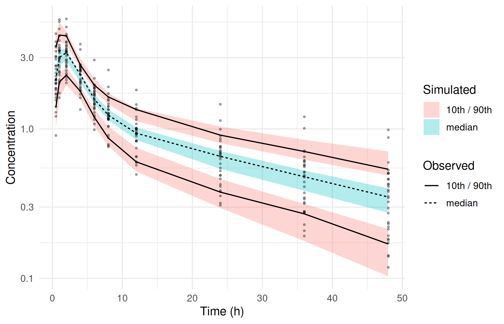

Figure 8.1: VPC of the base model: observed 10th, 50th and 90th percentiles (lines) with 90% intervals of the simulated percentiles (bands). Observations as points.

Read a VPC by checking whether each observed percentile line stays inside its simulated band. A line that leaves its band over a range of times points to a misspecification there: in structure, in variability (the outer percentiles) or in residual error.

Options that matter

Argument	Default	Meaning
`model`	—	Model file
`data`	`NULL`	Dataset providing subjects, doses and sampling times; `NULL` uses the model’s `[data]` block
`n_sim`	`1`	Number of replicates
`seed`	`42`	Random seed; the same seed gives identical results
`fit`	`NULL`	Fitted model whose `theta`, `omega` and `sigma` are used; `NULL` uses the model file’s initial values

match (propensity-score matching of the random effects to the observed design) and horizon (censoring time for time-to-event simulation) are covered in Simulating scenarios and Time-to-event models.

With a fixed seed, a simulation is reproducible:

identical(ferx_simulate(base$model, base$data, n_sim = 5, seed = 1, fit = fit),
          ferx_simulate(base$model, base$data, n_sim = 5, seed = 1, fit = fit))
#> [1] TRUE

Variants

Forgetting `fit`

Without fit, ferx_simulate() simulates from the model file’s initial values, not the estimates. A VPC then evaluates the starting values, not the model:

sim_inits <- ferx_simulate(base$model, base$data, n_sim = 500, seed = 1)
vpc_inits <- vpc_summary(obs, sim_inits, breaks)
vpc_plot(vpc_inits, obs)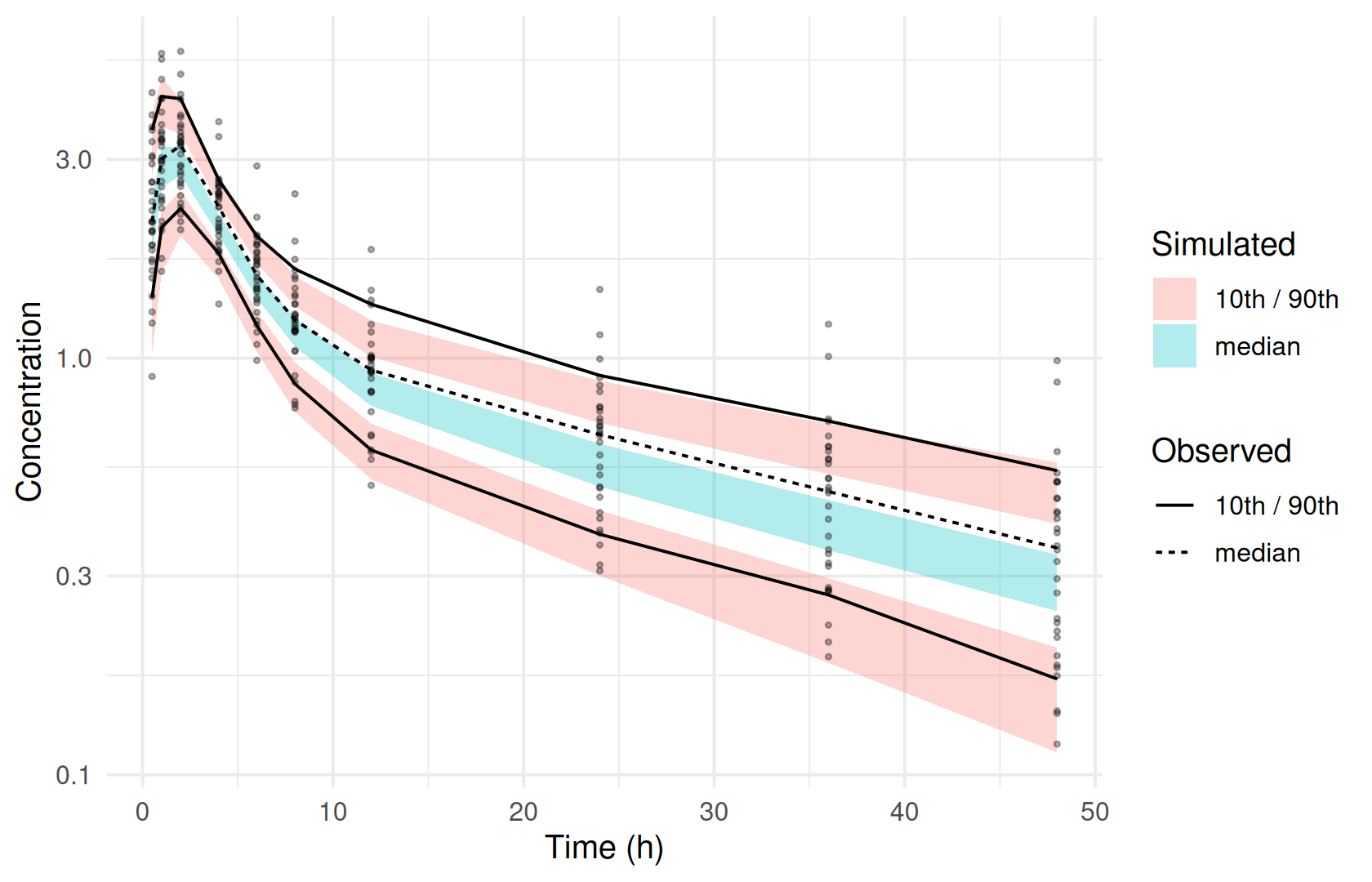

Figure 8.2: The same VPC simulated from the model file’s initial values instead of the fitted parameters.

Counting the bins in which the observed median lies outside its simulated band makes the difference concrete:

median_outside <- function(v) with(v[v$prob == 0.5, ], sum(value < lo | value > hi))
c(fitted = median_outside(vpc), initial_values = median_outside(vpc_inits), bins = length(breaks) - 1)
#>         fitted initial_values           bins 
#>              0              6             10

Pitfalls

Always pass fit when the simulation should reflect the estimates.
Simulated rows must match observed rows. Rows with MDV = 1 are never simulated. If the dataset has observation rows with an empty DV, ferx_simulate() simulates them (an empty DV means “simulate here”) but a fit skips them. ferx_simulate() reports this in simulation_warnings, and such rows have no counterpart in the observed data.
Binning drives the picture. Too few bins hide misfit and too many make the percentiles noisy. Check the number of observations per bin.
Doses and design differ between subjects. If they vary widely, stratify the VPC (for example by dose group) or use prediction-corrected percentiles, so that the design does not dominate the spread.

Summary

ferx_simulate(model, data, n_sim, seed, fit) replicates the study under the fitted model.
A VPC compares observed percentiles with intervals of simulated percentiles per time bin; a few lines of dplyr and ggplot2 build it.
Pass fit, set seed, and choose bins that follow the sampling design.

Next: Model development and selection compares and searches candidate models.

Reference

R help: ?ferx_simulate
ferx-core: simulation

Where you are

The data

Minimal runnable call

Reading the result: building a VPC

Options that matter

Variants

Forgetting fit

Pitfalls

Summary

Forgetting `fit`