Tables and figures

Where you are

The analysis is done: the final covariate model is fitted, evaluated and its uncertainty known. A report needs a parameter table, a record of the models compared, exposure metrics for the subjects, and a small set of figures. ferx returns all results as ordinary R data frames and lists, so reporting is plain R (dplyr, gt, ggplot2). The one ferx-specific tool is the model file’s [derived] and [output] blocks, which let the engine compute per-subject exposure metrics.

The data

cov <- ferx_example("two_cpt_oral_cov")
base <- ferx_example("two_cpt_oral_base")
fit <- ferx_fit(cov$model, cov$data, verbose = FALSE)
fit_base <- ferx_fit(base$model, base$data, verbose = FALSE)

Minimal runnable call: the parameter table

fit$estimates holds everything a parameter table needs. Between-subject variances are reported as coefficients of variation. For the log-normal random effects of this model, CV% = 100 × sqrt(exp(ω²) − 1), the value print() on the fit shows. Shrinkage comes from fit$shrinkage_eta.

That formula belongs to the log-normal form, so check what the etas are before applying it to every omega row (Initial estimates and a first fit):

table(fit$eta_param_types)
#> 
#> log_normal 
#>          5

All of them here. A logit-normal parameter is the case to watch: its distribution is asymmetric, so a CV% computed this way would misdescribe it. Report the variance on the logit scale, or a percentile range on the natural scale, instead.

est <- fit$estimates
omega_rows <- est$transform == "variance"
shrinkage <- setNames(100 * fit$shrinkage_eta, fit$eta_names)

param_table <- est |>
  mutate(
    type = case_when(omega_rows ~ "Between-subject variability (CV%)",
                     transform == "identity" ~ "Fixed effects",
                     TRUE ~ "Residual error"),
    value = ifelse(omega_rows, 100 * sqrt(exp(estimate) - 1), estimate),
    ci = ifelse(omega_rows, NA,
                sprintf("%s – %s", signif(lower_95, 3), signif(upper_95, 3))),
    shrinkage = ifelse(omega_rows, shrinkage[param], NA)
  ) |>
  select(type, param, value, rse_pct, ci, shrinkage)

param_table |>
  gt::gt(groupname_col = "type", rowname_col = "param") |>
  gt::fmt_number(columns = value, n_sigfig = 3) |>
  gt::fmt_number(columns = c(rse_pct, shrinkage), decimals = 1) |>
  gt::sub_missing(missing_text = "") |>
  gt::cols_label(value = "Estimate", rse_pct = "RSE (%)", ci = "95% CI", shrinkage = "Shrinkage (%)")

Table 12.1: Parameter estimates of the final covariate model.

	Estimate	RSE (%)	95% CI	Shrinkage (%)
Fixed effects
TVCL	4.95	7.3	4.24 – 5.65
TVV1	48.6	6.1	42.8 – 54.4
TVQ	9.58	4.3	8.78 – 10.4
TVV2	94.2	3.6	87.5 – 101
TVKA	1.26	7.8	1.06 – 1.45
THETA_WT	0.653	36.1	0.191 – 1.12
THETA_CRCL	0.565	39.2	0.13 – 0.999
Between-subject variability (CV%)
ETA_CL	33.7	26.1		0.3
ETA_V1	33.5	27.0		2.7
ETA_Q	22.9	27.3		2.2
ETA_V2	19.7	27.2		2.0
ETA_KA	43.8	27.7		3.6
Residual error
PROP_ERR	0.0196	5.7	0.0174 – 0.0218

Check the CV% column against the printout of the fit, which reports the same values:

round(param_table$value[omega_rows], 1)
#> [1] 33.7 33.5 22.9 19.7 43.8
grep("CV%", capture.output(print(fit)), value = TRUE)[1:2]
#> [1] "  ETA_CL                   [log-normal]  = 0.107531  CV% = 33.7  SE = 0.028096"
#> [2] "  ETA_V1                   [log-normal]  = 0.106348  CV% = 33.5  SE = 0.028678"

Reading the result: a model comparison table

A report also records the models that led to the final one. The fit objects carry all the numbers:

run_row <- function(f, description) {
  data.frame(model = f$model_name, description = description, method = f$method,
             converged = f$converged, parameters = f$n_parameters, ofv = f$ofv,
             aic = f$aic, bic_mixed = ferx_bic(f, "mixed"))
}
runs <- rbind(run_row(fit_base, "two-compartment, no covariates"),
              run_row(fit, "WT on CL and V1, CRCL on CL"))
runs$d_ofv <- runs$ofv - runs$ofv[1]
gt::gt(runs) |> gt::fmt_number(columns = c(ofv, aic, bic_mixed, d_ofv), decimals = 1)

Table 12.2: Models compared during development.

model	description	method	converged	parameters	ofv	aic	bic_mixed	d_ofv
two_cpt_oral_base	two-compartment, no covariates	FOCEI	TRUE	11	−1,185.4	−1,163.4	−1,145.7	0.0
two_cpt_oral_cov	WT on CL and V1, CRCL on CL	FOCEI	TRUE	13	−1,199.3	−1,173.3	−1,152.8	−13.9

Exposure metrics with `[derived]` and `[output]`

Maturity: beta

ferx-core labels [derived] and [output] beta. See feature maturity.

A [derived] block defines extra columns that the engine computes from each subject’s fitted profile and writes to fit$sdtab. [output] adds individual parameters or covariates to sdtab. The bundled two_cpt_oral_derived example shows the kinds of expression: per-row values (rate constants), per-subject aggregates (max, tmax) and integrals, including a periodic AUC per dosing window:

drv <- ferx_example("two_cpt_oral_derived")
invisible(ferx_model_get_section(drv$model, "derived"))
#> # [derived]
#>   K10 = CL / V1
#>   K12 = Q  / V1
#>   K21 = Q  / V2
#> 
#>   CMAX       = max(IPRED)
#>   TMAX       = tmax(IPRED)
#>   AUC_0_168  = integral(IPRED, from=0, to=168, step=0.2)
#>   AUC_TAU    = integral(IPRED, window=24, anchor=0, step=0.2)
invisible(ferx_model_get_section(drv$model, "output"))
#> # [output]
#>   CL V1 Q V2 KA
fit_drv <- ferx_fit(drv$model, drv$data, verbose = FALSE)
setdiff(names(fit_drv$sdtab), names(fit$sdtab))
#>  [1] "CL"        "V1"        "Q"         "V2"        "KA"        "K10"      
#>  [7] "K12"       "K21"       "CMAX"      "TMAX"      "AUC_0_168" "AUC_TAU"
fit_drv$sdtab |> filter(ID == 1) |> select(TIME, K10, CMAX, TMAX, AUC_TAU)
#>    TIME       K10     CMAX TMAX  AUC_TAU
#> 1   0.5 0.1245657 4.214751    1 35.68941
#> 2   1.0 0.1245657 4.214751    1 35.68941
#> 3   2.0 0.1245657 4.214751    1 35.68941
#> 4   4.0 0.1245657 4.214751    1 35.68941
#> 5   6.0 0.1245657 4.214751    1 35.68941
#> 6   8.0 0.1245657 4.214751    1 35.68941
#> 7  12.0 0.1245657 4.214751    1 35.68941
#> 8  24.0 0.1245657 4.214751    1 11.63592
#> 9  36.0 0.1245657 4.214751    1 11.63592
#> 10 48.0 0.1245657 4.214751    1  8.20865

CMAX and TMAX have one value per subject, repeated on every row. AUC_TAU has one value per 24-hour window.

The same blocks can be added to the final model. ferx_model_set_section() only replaces existing blocks, so append them to a copy of the model file:

report_dir <- book_tempdir("report")
exposure_model <- file.path(report_dir, "final_with_exposure.ferx")
writeLines(c(readLines(cov$model), "",
             "[derived]",
             "  CMAX = max(IPRED)",
             "  TMAX = tmax(IPRED)",
             "  AUC_0_48 = integral(IPRED, from=0, to=48, step=0.1)",
             "",
             "[output]",
             "  CL V1 WT CRCL"), exposure_model)
fit_exposure <- ferx_fit(exposure_model, cov$data, verbose = FALSE)
all.equal(fit_exposure$ofv, fit$ofv)
#> [1] TRUE

Derived columns do not change the estimation. The OFV is identical. One row per subject gives the exposure table:

exposure <- fit_exposure$sdtab |>
  distinct(ID, CL, V1, WT, CRCL, CMAX, TMAX, AUC_0_48)
head(exposure)
#>   ID       CL       V1   WT  CRCL     CMAX TMAX AUC_0_48
#> 1  1 4.360698 42.75776 70.6  73.7 4.134007    1 46.05033
#> 2  2 5.971806 60.81853 80.9  80.7 3.222542    1 36.35207
#> 3  3 4.944089 50.23567 90.7  99.1 3.274867    2 43.58047
#> 4  4 3.055909 21.72424 75.7  51.3 5.475072    2 60.77471
#> 5  5 5.824481 40.27095 86.5 124.0 3.452935    1 40.04630
#> 6  6 7.727280 45.64974 71.2 129.5 3.434671    1 29.04905

exposure |>
  mutate(weight_group = cut(WT, c(0, 60, 80, Inf), labels = c("< 60 kg", "60–80 kg", "> 80 kg"))) |>
  group_by(weight_group) |>
  summarise(n = n(), across(c(CMAX, AUC_0_48), list(median = median, min = min, max = max))) |>
  gt::gt() |>
  gt::fmt_number(columns = -c(weight_group, n), n_sigfig = 3)

Table 12.3: Individual exposure after a single 250 mg dose, summarised by body weight group.

weight_group	n	CMAX_median	CMAX_min	CMAX_max	AUC_0_48_median	AUC_0_48_min	AUC_0_48_max
< 60 kg	4	3.58	2.95	4.15	50.6	45.0	83.5
60–80 kg	17	3.36	2.32	5.48	43.8	29.0	65.3
> 80 kg	9	3.22	2.10	3.45	36.6	26.9	52.3

Figures for a report

Plot figures with one consistent style. A four-panel goodness-of-fit figure:

library(patchwork)
sd <- fit$sdtab
identity_panel <- function(x, xlab) {
  ggplot(sd, aes({{ x }}, DV)) +
    geom_abline(linetype = "dashed") + geom_point(alpha = 0.4, size = 1) +
    geom_smooth(method = "loess", formula = y ~ x, se = FALSE, linewidth = 0.6) +
    scale_x_log10() + scale_y_log10() + labs(x = xlab, y = "Observed")
}
residual_panel <- function(x, xlab) {
  ggplot(sd, aes({{ x }}, CWRES)) +
    geom_hline(yintercept = c(-2, 0, 2), linetype = c("dotted", "dashed", "dotted")) +
    geom_point(alpha = 0.4, size = 1) +
    geom_smooth(method = "loess", formula = y ~ x, se = FALSE, linewidth = 0.6) + labs(x = xlab)
}
gof <- (identity_panel(PRED, "Population prediction") | identity_panel(IPRED, "Individual prediction")) /
  (residual_panel(TIME, "Time (h)") | residual_panel(PRED, "Population prediction")) +
  plot_annotation(tag_levels = "A")
gof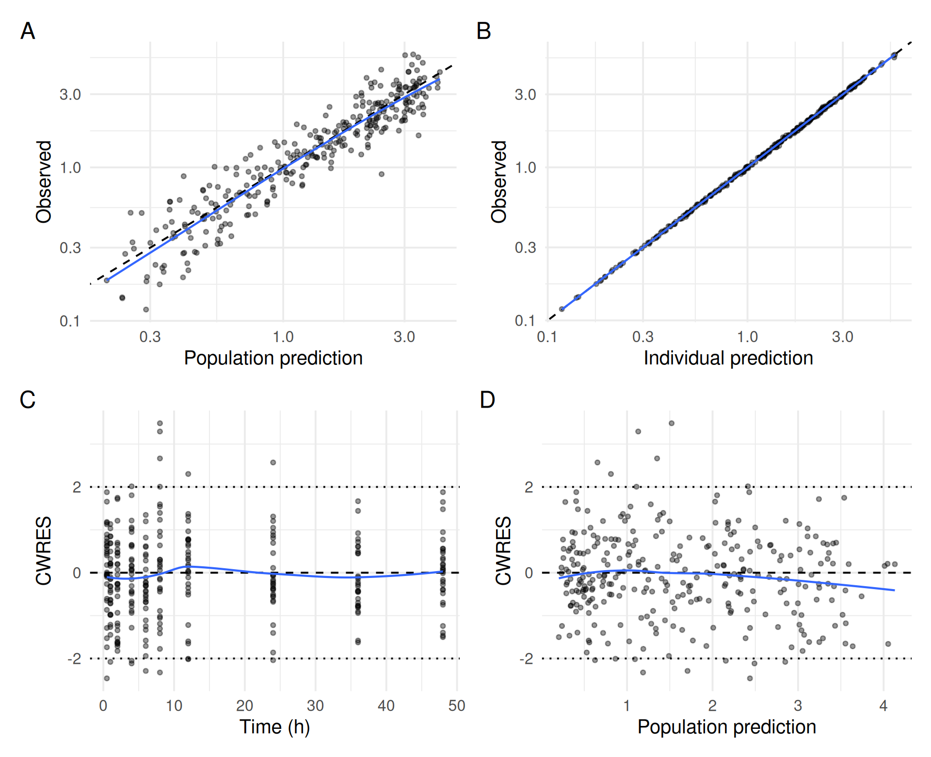

Figure 12.1: Goodness of fit of the final model.

And the covariate relationship the final model contains, with individual clearances against creatinine clearance and the typical curve for a 70 kg subject from the estimates:

theta <- fit$theta
typical_cl <- data.frame(CRCL = seq(40, 160, length.out = 100)) |>
  mutate(CL = theta[["TVCL"]] * (CRCL / 100)^theta[["THETA_CRCL"]])
cl_plot <- ggplot(exposure, aes(CRCL, CL)) +
  geom_point(aes(size = WT), alpha = 0.6) +
  geom_line(data = typical_cl) +
  labs(x = "Creatinine clearance", y = "Clearance (individual)", size = "Weight (kg)")
cl_plot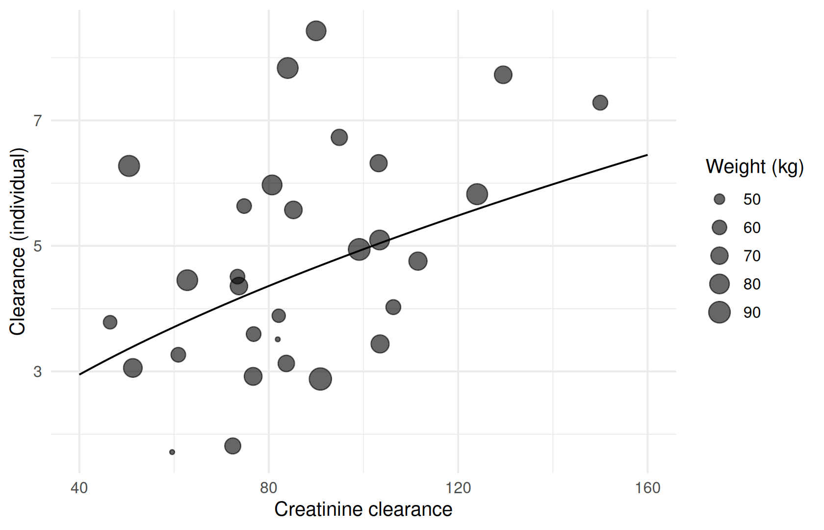

Figure 12.2: Individual clearance against creatinine clearance, with the typical relationship for a 70 kg subject.

The typical curve uses the model’s CL = TVCL * (WT / 70)^THETA_WT * (CRCL / 100)^THETA_CRCL at WT = 70 (see ferx_model_get_section(cov$model, "individual_parameters")).

Save figures and tables in the formats your report needs:

ggsave(file.path(report_dir, "gof.png"), gof, width = 8, height = 6.5, dpi = 300)
ggsave(file.path(report_dir, "cl_crcl.pdf"), cl_plot, width = 6, height = 4)
write.csv(exposure, file.path(report_dir, "exposure.csv"), row.names = FALSE)
list.files(report_dir)
#> [1] "cl_crcl.pdf"              "exposure.csv"            
#> [3] "final_with_exposure.ferx" "gof.png"

Options that matter

[derived] expressions (full syntax on the ferx-core derived page):

Kind	Example	Result
Per row	`K10 = CL / V1`	One value per observation row
Aggregate	`CMAX = max(IPRED)`, `TMAX = tmax(IPRED)`, `CTROUGH = min(IPRED, TAD < 1e-10)`	One value per subject, optionally over a filter
Integral	`AUC = integral(IPRED, from=0, to=24, step=0.1)`	Area over an interval
Periodic integral	`AUC_TAU = integral(IPRED, window=24, anchor=0, step=0.2)`	One area per dosing window
Compartment state	`C_PERIPH = peripheral`, `AUC_P = integral(compartments[2], from=0, to=48, step=0.1)`	A state of the model (differs between analytical and ODE models, Model states in [derived])

[output] lists individual parameters, covariates or [derived] expressions to add to sdtab (ferx-core output page). A theta is none of those, and asking for one stops the fit:

theta_out <- file.path(report_dir, "output_theta.ferx")
writeLines(c(readLines(base$model), "", "[output]", "  TVCL"), theta_out)
try(ferx_fit(theta_out, base$data, verbose = FALSE))
#> Error in ferx_rust_fit(model_path = normalizePath(model), data_path = normalizePath(data),  : 
#>   Fit error: [output] column `TVCL` is not recognised as a covariate, individual parameter, or derived expression. Known: WT, CRCL, CL, V1, Q, V2, KA, ID, TIME, DV, CENS, OCC, CMT, PRED, IPRED, CWRES, IWRES, NPDE, NPD, EBE_OFV, N_OBS, TAFD, TAD [E_OUTPUT_UNKNOWN_COLUMN]

Pitfalls

Integrals and sampling. Without step, an IPRED integral uses only observation times. With step, IPRED on the grid is approximated by the nearest observation-time value. Choose intervals covered by your sampling. AUC_0_48 matches the 48-hour sampling here; the bundled example’s AUC_0_168 extends beyond it.
Report variances on a clear scale. fit$estimates holds omega as variances and sigma as given by transform. State the scale or transformation in the table, as done here for CV%.
Derived names must not clash with built-in sdtab columns or with model parameter names.

Summary

Build parameter and model comparison tables from fit$estimates and the fit’s scalars with gt.
Let the engine compute exposure metrics with [derived], and add individual parameters and covariates to sdtab with [output].
Draw report figures from fit$sdtab and derived data frames, and save them with ggsave().

Next: Reproducibility and sharing saves the fit and makes the analysis reproducible.

Reference

R help: ?ferx_fit (estimates, sdtab, shrinkage_eta), ?ferx_bic
ferx-core: [derived], [output]

Where you are

The data

Minimal runnable call: the parameter table

Reading the result: a model comparison table

Exposure metrics with [derived] and [output]

Figures for a report

Options that matter

Pitfalls

Summary

Exposure metrics with `[derived]` and `[output]`