Diagnosing the model

Where you are

A converged fit with a sensible OFV is only a candidate. Before trusting it, check whether the model describes the data: are predictions unbiased, are residuals structureless, are the random effects well behaved and informed by the data, and are the parameters identifiable? This chapter works through these checks for the base model. It uses the fit object’s tables and plain ggplot2, plus the simulation-based NPDE.

The data

base <- ferx_example("two_cpt_oral_base")
fit <- ferx_fit(base$model, base$data, verbose = FALSE)

Minimal runnable call

Most diagnostics come straight from fit$sdtab, which has one row per observation:

head(fit$sdtab)
#>   ID TIME     DV     PRED    IPRED      CWRES      IWRES   EBE_OFV N_OBS TAFD
#> 1  1  0.5 3.5262 2.223319 3.538980  0.8812067 -0.1840541 -40.00822    10  0.5
#> 2  1  1.0 4.1950 3.124361 4.134356  0.9840705  0.7476190 -40.00822    10  1.0
#> 3  1  2.0 3.3759 3.290091 3.438487 -1.5465219 -0.9277259 -40.00822    10  2.0
#> 4  1  4.0 2.1090 2.331357 2.085948  0.1373079  0.5632588 -40.00822    10  4.0
#> 5  1  6.0 1.4915 1.638392 1.485297  0.1491897  0.2128522 -40.00822    10  6.0
#> 6  1  8.0 1.1890 1.263978 1.212727 -0.8405074 -0.9972035 -40.00822    10  8.0
#>   TAD
#> 1 0.5
#> 2 1.0
#> 3 2.0
#> 4 4.0
#> 5 6.0
#> 6 8.0

PRED is the population prediction (all etas zero). IPRED is the individual prediction at the subject’s estimated random effects. CWRES and IWRES are the conditional weighted and individual weighted residuals. TAFD and TAD are time after first dose and time after dose.

Reading the result

Observations against predictions

fit$sdtab |>
  tidyr::pivot_longer(c(PRED, IPRED), names_to = "prediction", values_to = "value") |>
  ggplot(aes(value, DV)) +
  geom_abline(linetype = "dashed") +
  geom_point(alpha = 0.4) +
  geom_smooth(se = FALSE, method = "loess", formula = y ~ x) +
  scale_x_log10() + scale_y_log10() +
  facet_wrap(~prediction) +
  labs(x = "Prediction", y = "Observation")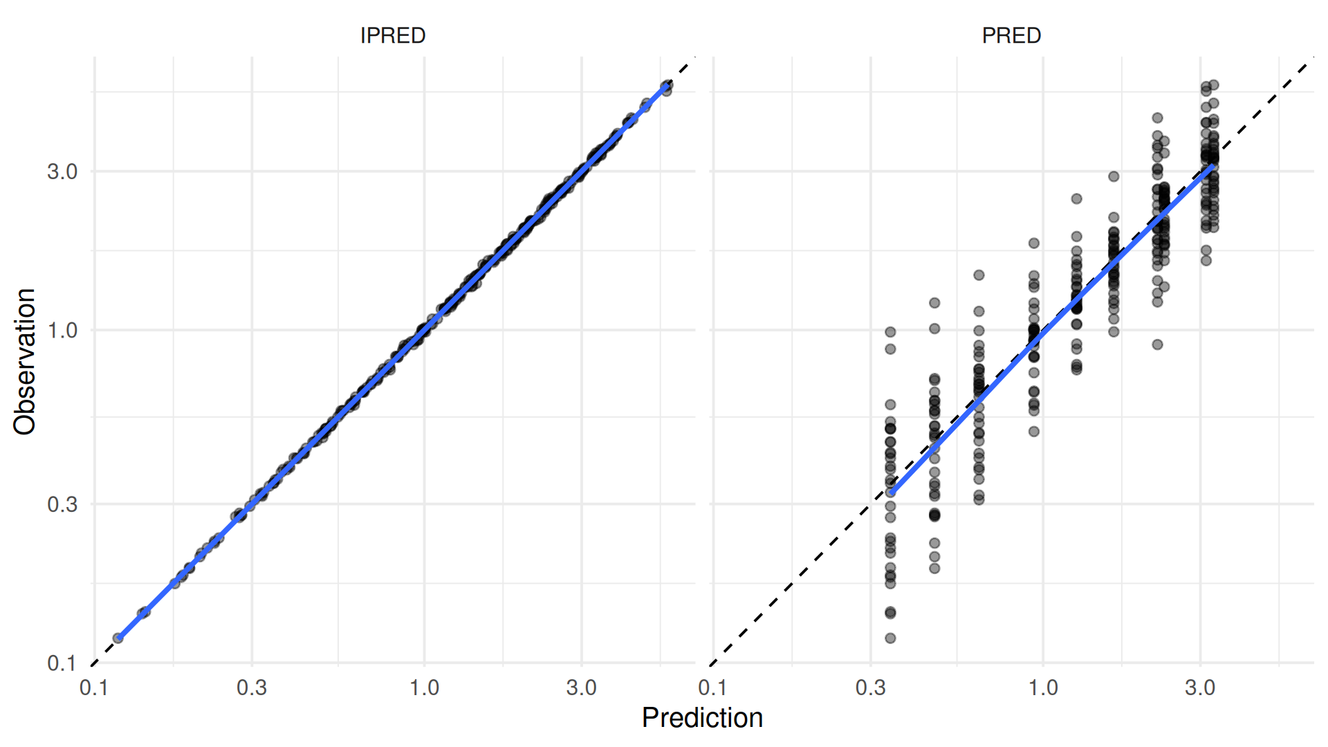

Figure 7.1: Observations against population and individual predictions (log scales), with a smooth.

Points should scatter around the identity line, and the smooth should follow it. Scatter around PRED also includes between-subject variability, so it is wider than around IPRED.

Residuals

library(patchwork)
res_plot <- function(x, y, xlab) {
  ggplot(fit$sdtab, aes({{ x }}, {{ y }})) +
    geom_hline(yintercept = 0, linetype = "dashed") +
    geom_point(alpha = 0.4) +
    geom_smooth(se = FALSE, method = "loess", formula = y ~ x) +
    labs(x = xlab)
}
res_plot(TIME, CWRES, "Time (h)") + res_plot(PRED, CWRES, "PRED") + res_plot(IPRED, IWRES, "IPRED")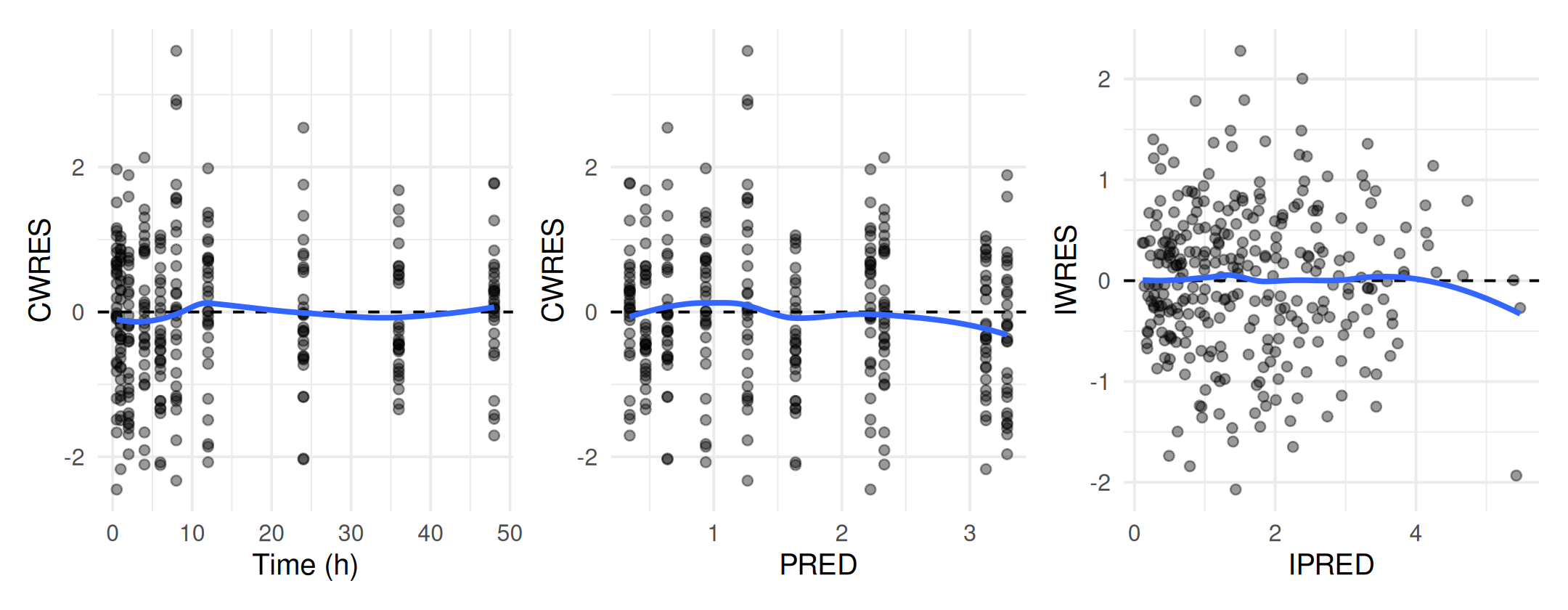

Figure 7.2: CWRES against time and against population prediction; IWRES against individual prediction.

Residuals should be centred on zero with no trend over time or predictions. Most should fall within ±2, and the spread should not change with the prediction. Under a correct model CWRES are roughly standard normal:

ggplot(fit$sdtab, aes(sample = CWRES)) +
  stat_qq(alpha = 0.5) +
  stat_qq_line() +
  labs(x = "Theoretical quantile", y = "CWRES")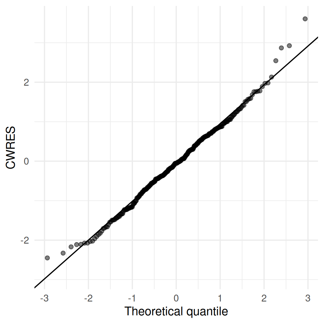

Figure 7.3: Normal quantile plot of CWRES.

The fit also tests the residuals for serial correlation within subjects. fit$dw_statistic is the Durbin-Watson statistic of the individual residuals (2.91 here) and fit$iwres_lag1_r their lag-1 correlation (-0.53). Values far from 2 and 0 respectively trigger the dw_autocorrelation warning this fit carries. The statistic reads in two directions, and they mean opposite things:

`dw_statistic`	Reading	Usually points at
below 1.5	Positive autocorrelation	Missing dynamics: a delay the model does not have, an absorption phase too simple, variability between occasions
1.5 to 2.5	No serial correlation worth acting on	–
above 2.5	Negative autocorrelation	Over-parameterisation, or a residual error model that does not fit the data

ferx_get_warnings(fit)
#> ferx fit warnings  (two_cpt_oral_base)
#> -------------------------------------------------
#> [WARNING]  dw_autocorrelation
#>             Negative IWRES autocorrelation detected (Durbin-Watson = 2.91).
#>             Possible over-parameterization or misspecified error model.
#>             Negative IWRES autocorrelation suggests over-parameterisation or a
#>             misspecified error model. Consider removing a parameter or
#>             simplifying the residual model.
#> 
#> -------------------------------------------------
#> 0 CRITICAL   1 WARNING   0 INFO

ferx suggests over-parameterisation or a misspecified residual error model as possible causes. Model development and selection tests alternative residual error models systematically with ferx_ruvsearch().

Individual fits

fit$sdtab |>
  filter(ID %in% unique(ID)[1:9]) |>
  ggplot(aes(TIME)) +
  geom_point(aes(y = DV)) +
  geom_line(aes(y = IPRED)) +
  geom_line(aes(y = PRED), linetype = "dashed") +
  scale_y_log10() +
  facet_wrap(~ID) +
  labs(x = "Time (h)", y = "Concentration")

Figure 7.4: Observations (points) with individual (solid) and population (dashed) predictions for the first nine subjects.

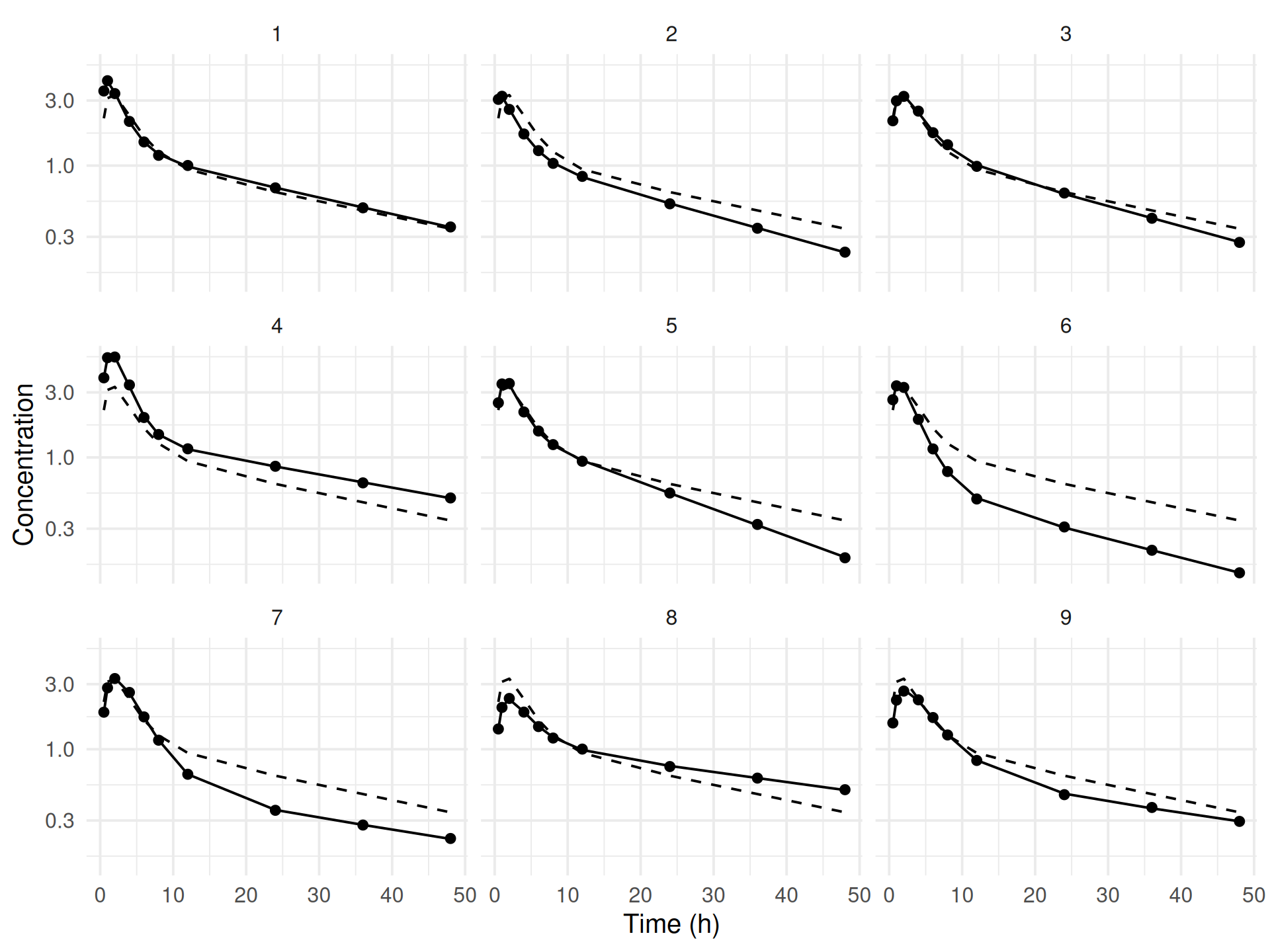
These lines connect predictions at the observation times only. For smooth curves between samples, predict on a dense time grid with ferx_predict() (Simulating scenarios).

Random effects and shrinkage

fit$ebe_etas holds each subject’s estimated random effects:

fit$ebe_etas |>
  tidyr::pivot_longer(-ID, names_to = "eta") |>
  ggplot(aes(value)) +
  geom_histogram(bins = 12) +
  geom_vline(xintercept = 0, linetype = "dashed") +
  facet_wrap(~eta, nrow = 1)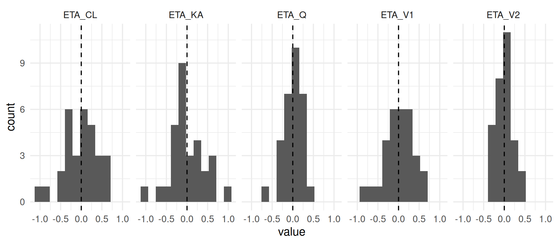

Figure 7.5: Distribution of the estimated random effects.

Shrinkage measures how strongly the individual estimates are pulled towards zero. High eta shrinkage means the data carry little information about that random effect for individual subjects, which makes eta-based plots (including the covariate plots below) unreliable for that parameter:

data.frame(eta = fit$eta_names, shrinkage_pct = round(100 * fit$shrinkage_eta, 1))
#>      eta shrinkage_pct
#> 1 ETA_CL          -0.2
#> 2 ETA_V1           3.6
#> 3  ETA_Q           2.9
#> 4 ETA_V2           2.4
#> 5 ETA_KA           4.2
c(eps_shrinkage_pct = round(100 * fit$shrinkage_eps, 1))
#> eps_shrinkage_pct 
#>              27.9

fit$eta_normality holds a Shapiro-Wilk test per eta. A flag marks p < 0.05:

fit$eta_normality
#>      eta     W  p_val flag
#> 1 ETA_CL 0.964 0.3878     
#> 2 ETA_V1 0.975 0.6775     
#> 3  ETA_Q 0.986 0.9534     
#> 4 ETA_V2 0.977 0.7454     
#> 5 ETA_KA 0.978 0.7739

Random effects and covariates

fit$eta_cov correlates each eta with each subject-level numeric covariate in the dataset, sorted by descending |r|, and marks the pairs worth following up in its flag column at |r| >= 0.3. It is a quick first look for covariate relationships, and it is NULL when the model declares no etas, the dataset carries no usable numeric covariate, or the data file can no longer be read from fit$data_path:

fit$eta_cov
#>       eta covariate      r  p_val flag
#> 1  ETA_CL      CRCL  0.469 0.0090  [!]
#> 2  ETA_CL        WT  0.382 0.0371  [!]
#> 3  ETA_V1        WT  0.305 0.1010  [!]
#> 4  ETA_KA        WT  0.133 0.4821     
#> 5   ETA_Q        WT  0.117 0.5388     
#> 6  ETA_V2      CRCL  0.086 0.6503     
#> 7  ETA_V2        WT  0.081 0.6688     
#> 8  ETA_V1      CRCL  0.062 0.7463     
#> 9   ETA_Q      CRCL  0.045 0.8136     
#> 10 ETA_KA      CRCL -0.002 0.9899
with(fit$eta_cov, range(abs(r)[nzchar(trimws(flag))]))
#> [1] 0.305 0.469

subjects <- read.csv(base$data, na.strings = ".") |> distinct(ID, WT, CRCL)
fit$ebe_etas |>
  mutate(ID = as.integer(ID)) |>
  left_join(subjects, by = "ID") |>
  tidyr::pivot_longer(c(WT, CRCL), names_to = "covariate", values_to = "value") |>
  ggplot(aes(value, ETA_CL)) +
  geom_hline(yintercept = 0, linetype = "dashed") +
  geom_point() +
  geom_smooth(method = "lm", formula = y ~ x, se = FALSE) +
  facet_wrap(~covariate, scales = "free_x") +
  labs(x = NULL)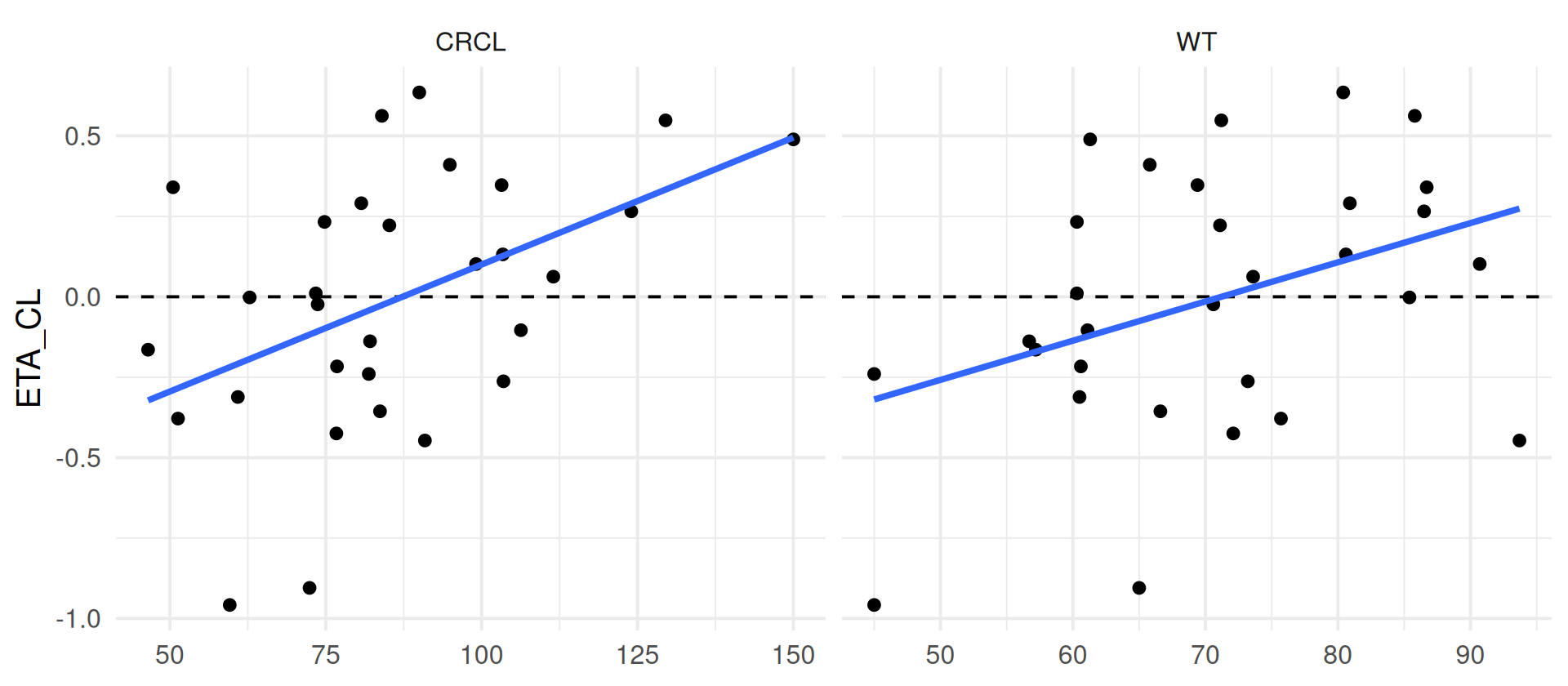

Figure 7.6: Clearance random effect against body weight and creatinine clearance.

ETA_CL has the strongest correlations here, with CRCL (r = 0.469) and WT (r = 0.382). That motivates the covariate search in Model development and selection. Covariate modeling covers covariate screening tools in more detail.

Parameter identifiability

The covariance step yields the parameter correlation matrix. Correlations near ±1 point to parameters the data cannot separate:

as.data.frame(as.table(fit$cor_matrix)) |>
  ggplot(aes(Var1, Var2, fill = Freq)) +
  geom_tile() +
  scale_fill_gradient2(limits = c(-1, 1)) +
  labs(x = NULL, y = NULL, fill = "r") +
  theme(axis.text.x = element_text(angle = 45, hjust = 1))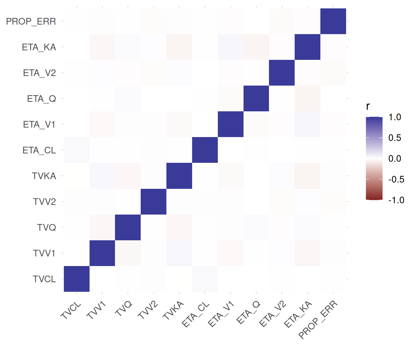

Figure 7.7: Correlation matrix of the parameter estimates.

c(max_abs_correlation = fit$max_abs_correlation, condition_number = fit$condition_number)
#> max_abs_correlation    condition_number 
#>          0.05013899          1.23482058

The condition number is the ratio of the largest to the smallest eigenvalue of this correlation matrix (fit$eigenvalues). ferx flags values above 1000.

NPDE

Normalized prediction distribution errors (NPDE) compare each observation with its distribution simulated under the fitted model. Unlike CWRES, they do not rely on a linearisation, and under a correct model they follow a standard normal distribution. ferx_calc_npde() computes them after the fit and returns the fit with NPDE and NPD columns added to sdtab:

fit <- ferx_calc_npde(fit, nsim = 1000, seed = 1)
summary(fit$sdtab[, c("NPDE", "NPD")])
#>       NPDE               NPD           
#>  Min.   :-3.29053   Min.   :-2.575829  
#>  1st Qu.:-0.65419   1st Qu.:-0.675277  
#>  Median :-0.01379   Median : 0.006267  
#>  Mean   : 0.04322   Mean   : 0.060819  
#>  3rd Qu.: 0.72004   3rd Qu.: 0.672132  
#>  Max.   : 2.57583   Max.   : 3.290527

(ggplot(fit$sdtab, aes(TIME, NPDE)) +
   geom_hline(yintercept = c(-1.96, 0, 1.96), linetype = c("dotted", "dashed", "dotted")) +
   geom_point(alpha = 0.4) +
   geom_smooth(se = FALSE, method = "loess", formula = y ~ x) +
   labs(x = "Time (h)")) +
  (ggplot(fit$sdtab, aes(sample = NPDE)) + stat_qq(alpha = 0.5) + stat_qq_line() +
     labs(x = "Theoretical quantile", y = "NPDE"))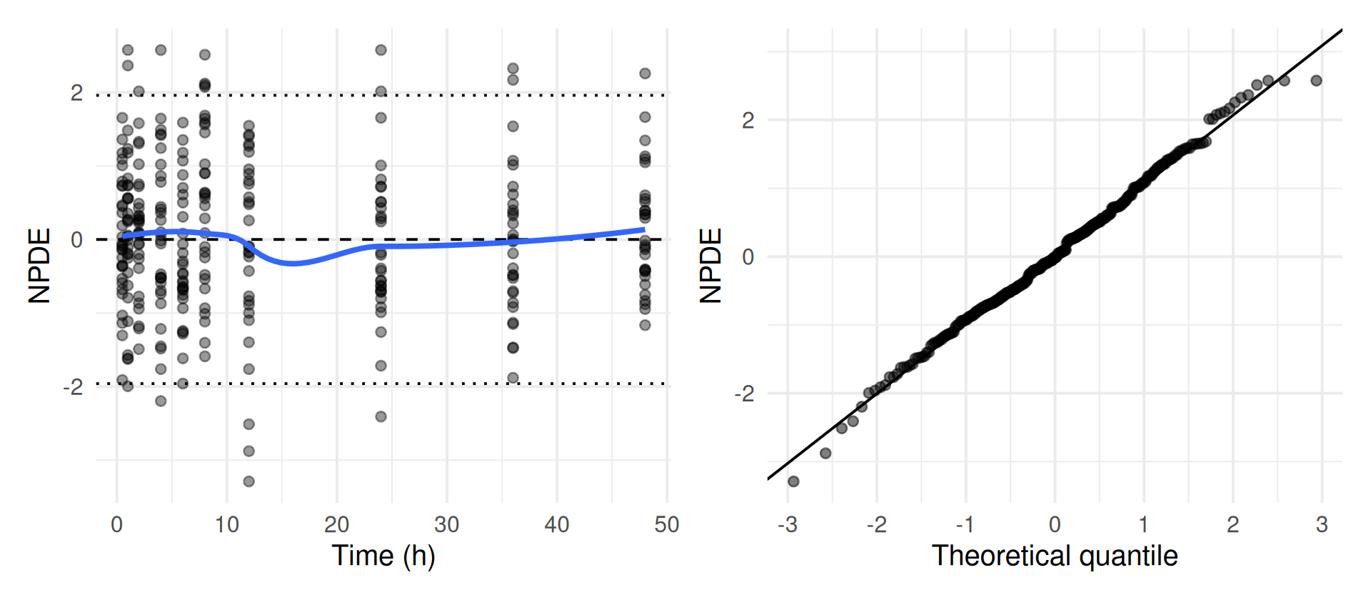

Figure 7.8: NPDE against time and their normal quantile plot.

nsim must exceed each subject’s number of observations; subjects that don’t get NA NPDE. seed makes the result reproducible. model and data default to the paths stored in the fit. NPDE can also be computed during the fit with the npde_nsim and npde_seed settings:

book_settings_table(c("npde_nsim", "npde_seed"))

Table 7.1

Setting	Values	Default	Description
`npde_nsim`	integer ≥ 0	`0`	Number of Monte-Carlo replicates per subject used to compute the simulation-based NPDE/NPD diagnostics after the fit.
`npde_seed`	integer	—	RNG seed for the NPDE/NPD simulation, for reproducible diagnostics.

Options that matter

Function	Argument	Meaning
`ferx_calc_npde()`	`fit`	The fit to evaluate
	`nsim`	Monte Carlo replicates per subject (default 1000)
	`seed`	Random seed (default: the engine’s)
	`model`, `data`	Override the model and data paths stored in the fit
`ferx_xpose()`	`fit`	Fit to convert
	`backend`	`"xpose"` (default) or `"xpose4"`
	`continuous`, `categorical`	Override which covariates are treated as continuous or categorical
	`runno`	Run number stored on the object
	`iterations`	Include the per-parameter optimizer trace (needs `optimizer_trace = TRUE`)

Using xpose

ferx_xpose() converts a fit into a data object for the xpose (or xpose4) diagnostics packages, which provide ready-made goodness-of-fit, parameter and covariate plots. It maps sdtab, the individual parameters, the random effects and the covariates to xpose’s tables. xpose is not a dependency of this book, so the code is not run here:

fit_trace <- ferx_fit(base$model, base$data, optimizer_trace = TRUE, verbose = FALSE)
xpdb <- ferx_xpose(fit_trace, backend = "xpose", runno = 1, iterations = TRUE)
xpose::dv_vs_ipred(xpdb)
xpose::prm_vs_iteration(xpdb)   # parameter values over the optimizer trace

Pitfalls

Shrinkage limits eta-based diagnostics. When eta shrinkage is high, eta histograms and eta-covariate plots mostly show the prior, not the data.
Small negative shrinkage is possible. ETA_CL shows -0.2% here; this is not an error.
The plotted lines are not the model curve. sdtab has predictions only at observation times. Use ferx_predict() on a dense grid for smooth individual curves.
fit$eta_cov is a screen, not a test of a covariate model. Confirm relationships by fitting covariate models (Model development and selection).

Warnings you may see here

See the ferx-core warnings page for details.

dw_autocorrelation (warning): the individual residuals are autocorrelated (Durbin-Watson out of range). Revisit the residual error or structural model.
eta_normality (warning): an eta departs from normality.
eps_shrinkage (warning): residual shrinkage is high or negative. Sparse data for the error model; consider simplifying it.
eta_shrinkage (warning): one or more eta shrinkages exceed about 30%. The data poorly inform that variability.
boundary_estimate (warning): a theta estimate sits at a bound. Relax the bound or simplify the model.
inflated_rse (warning): a theta has a relative standard error above about 50%.
high_correlation (warning): a pair of thetas has |correlation| ≥ 0.95.
condition_number (critical): the covariance matrix is ill-conditioned. The model is likely over-parameterised.

Initial estimates and a first fit shows a fit that carries several of these at once.

Summary

Plot fit$sdtab: observations against predictions, residuals against time and predictions, and individual fits.
Check random effects with fit$ebe_etas, shrinkage and fit$eta_normality. Use fit$eta_cov for a first covariate screen.
Check identifiability with fit$cor_matrix and the condition number.
Add simulation-based NPDE with ferx_calc_npde(). Use ferx_xpose() if you work with xpose.

Next: Simulation-based evaluation: VPC evaluates the model by simulation.

Reference

R help: ?ferx_calc_npde, ?ferx_xpose, ?ferx_fit (the sdtab, eta_cov, eta_normality, cor_matrix elements)
ferx-core: output files and sdtab, warnings